Downscaling

Global climate models (GCMs) are our best tools for providing climate projections. A climate model is a mathematical representation of the climate system.

Mathematical equations are solved on a super-computer at points on a 3-dimensional grid in the ocean and atmosphere, over a number of time-steps. Due to practical computing constraints, the spatial resolution (horizontal size of grid-cells) is about 200 km.

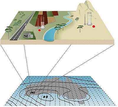
‘Downscaling’ is the process by which coarse-resolution GCM outputs are translated into finer resolution climate information, so that they better account for regional climatic influences, such as local topography.

There are many different ways in which GCM outputs can be translated to finer resolutions or even point locations. As a general guide, downscaling methods can typically be categorised into three groups: change factor methods, statistical downscaling and dynamical downscaling.

Change factor methods are techniques of combining the coarse-resolution change ‘signal’ from GCM outputs with finer-resolution observed datasets. This method is quick and convenient and produces data that look like observations. This method has been used to create application-ready data for Australia. However it is important to remember that this method cannot reveal new regional detail in the GCM climate change signal - the extra detail comes from the finer resolution in the underlying observed climate dataset.

SOURCE: Bureau of Meteorology

Statistical and dynamical downscaling are more technical processes than change factor methods, and have the potential to reveal new and plausible regional detail in the climate change signal.

For the statistical downscaling method, observed relationships between local synoptic situations and the large-scale climate are used to build the statistical model. This usually leads to a very close representation of the observed climate in the statistical downscaling model, (almost) independent of the choice of host global climate model. The model can then be used to infer local-scale changes from large-scale changes generated by GCMs.

Dynamical downscaling involves running a climate model at fine resolution using the GCM to provide the large-scale boundary conditions. Some dynamical downscaling is done globally, and some is done regionally using regional climate models (RCMs). Monthly sea-surface temperature (SST) data from a global climate model simulation typically provide boundary conditions. The SSTs are initially adjusted to match the observed mean climate before being used in downscaling (called SST-bias adjustment). This means the resulting dynamically downscaled simulations are again fairly similar to each other and to the observations over the historical period (1986-2005).

We expect statistical and dynamical downscaling to have the most potential to reveal regional detail in the change signal in areas where there are marked regional climate contrasts due to local features such as complex topography or coastlines. This extra information about climate change is termed ‘added value’. For example, it may be plausible to get a different rainfall change on one side of a mountain range than the other due to different topographic affects arising from changes in atmospheric circulation. Therefore, in Australia we expect downscaling techniques to have most added value in areas such as Tasmania, around the Australian Alps and Great Dividing Ranges, the east coast of NSW and some regions of southwest Western Australia.

Results from statistical and dynamical downscaling complement GCM results, where it is likely to show ‘added value’ in the climate change signal of rainfall and temperature.