Climate Change in Australia
Climate information, projections, tools and data
KEY CONCEPTS
The ESCI Climate Risk Assessment Framework recommends a quantitative approach which relies on future climate projections derived from global climate models (GCMs).
GCMs are mathematical representations of the climate system run on powerful supercomputers and based on the laws of physics. (GCMs are closely related to models used for daily weather prediction.)
The underpinning science is complex, so ESCI Key Concept fact sheets provide guidance on specific topics, tailored for the electricity sector to support the use of climate information as part of a risk assessment.
Choosing Representative Emissions Pathways (RCPs)
- Scenario Analysis
- Selecting Different Pathways for the Electricity Sector
- Available Data from the ESCI Project
- Considering Lower Emissions Pathways
- References
- Downloads
Scenario analysis
Assessing the impact of climate change on investment decisions requires practitioners to make choices about what the future may look like. To understand how our climate may change in future it is useful to undertake a scenario analysis. According to the Australian Institute for Disaster Resilience,1 hazard scenarios should ‘explore probable, plausible, possible and even preposterous hazard futures. They raise awareness, stretch current thinking, stress-test current practices and catalyse actions to reduce the possibility of “inevitable surprises."’
The development of scenarios that are targeted at managing climate risk is an evolving area, with new developments such as Network for Greening the Financial System (NGFS ) producing new scenario analyses that will be relevant moving forward, particularly around transition risks. However, detailed analysis and modelling for analysing physical risks is best done employing the international standard set of scenarios that are used in the set of mature climate modelling simulations, and regional downscaling from those simulations.
The climate change research community has developed a set of scenarios describing how the future may evolve in terms of socio-economic change, technological change, energy, land use, and emissions and atmospheric concentrations of greenhouse gases and air pollutants (van Vuuren et al. 2011). These scenarios are called ‘Representative Concentration Pathways’ or RCPs (Figure 1). The Intergovernmental Panel on Climate Change (IPCC) has modelled a number of RCPs (Table 1). The four most commonly used RCPs range from very high (RCP8.5) to very low (RCP2.6) future concentrations. The numerical values of the RCPs (2.6, 4.5, 6.0 and 8.5) refer to the radiative forcing (Watts per square metre) in 2100.2
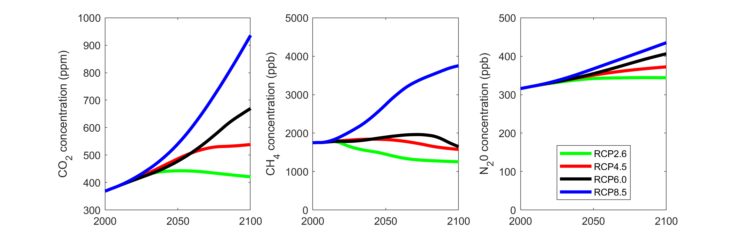
Figure 1 Four representative concentration pathways (RCPs) for carbon dioxide (CO2), methane (CH4) and nitrous oxide (N2O). (Source: van Vuuren et al. 2011 )
Selecting different pathways for the electricity sector
The Paris Agreement aims to limit global warming to well below 2 oC relative to pre-industrial (1850–1900) levels. This would require global CO2 emissions to decline rapidly towards net negative global emissions after 2050. Figure 2 shows how temperatures are projected to change for each pathway; RCP2.6 has a two-in-three chance of keeping global warming below 2 oC (IPCC 2019) . Figure 2 shows the relationship between RCPs.
Near-term:2031-2050 | End-of-century: 2081-2100 |
|||
|---|---|---|---|---|
Scenario | Mean (°C) | Likely range (°C) | Mean (°C) | Likely range (°C) |
RCP2.6 | 1.6 | 1.1 to 2.0 | 1.6 | 0.9 to 2.4 |
RCP4.5 | 1.7 | 1.3 to 2.2 | 2.5 | 1.7 to 3.3 |
RCP6.0 | 1.6 | 1.2 to 2.0 | 2.9 | 2.0 to 3.8 |
RCP8.5 | 2.0 | 1.5 to 2.4 | 4.3 | 3.2 to 5.4 |
")
Figure 2 Projected global temperature change for each representative concentration pathway. (Adapted from IPCC 2013)
It is strongly recommended that both low and high concentration pathways are used in climate risk assessments. If the climate risk assessment is part of a requirement for financial reporting, then the Taskforce on Climate-related Financial Disclosure3 recommends using scenarios that are consistent with a global warming of 2 oC and with a higher global warming (4 oC is commonly cited) by the year 2100. The Climate Measurement Standards Initiative (2020), developed by Australian finance representatives, recommends using RCP2.6 as an approximation for a 2 oC warming scenario and RCP8.5 for a 4 oC warming scenario. However, RCP4.5 can also be used for the 2 oC warming scenario if the focus is up to 2050 (see Figure 2). Note: historical cumulative carbon dioxide emissions are tracking close to RCP8.5 (Schwalm et al. 2020)4 but recent emissions, current policy and particularly the projected emissions according to Nationally Determined Contributions (NDCs) are now tracking below RCP8.5 and are more consistent with a medium to high pathway.
Available data from the ESCI project
The ESCI project has produced detailed modelling and data sets for two representative concentration pathways, relevant to adaptation planning in response to changing physical climate risks, including for climate risk ‘stress testing’:
- RCP8.5—a very high pathway where CO2 emissions continue to grow, consistent with ongoing high greenhouse gas emissions, 3–5 °C of global warming since pre-industrial times by 2100 (or even more), extremely large physical risk challenges and lower transition risk challenges as the global economy fails to transition away from fossil fuels.
- RCP4.5—an intermediate pathway where CO2 emissions peak around 2040 then plateau and decline, consistent with 2–3 °C of global warming since pre-industrial times, with large physical risk challenges but also large transition risks.5
Sometimes there is a requirement for assessments of physical impacts at very low pathways where the world completely transitions away from fossil fuels and the Paris Agreement targets are met. These cases represent profound transition scenarios for the electricity sector, with high transition risk, but the physical risk challenges for these low pathways are lower than for RCP4.5 and RCP8.5.
Considering lower emissions pathways
RCP2.6 is a commonly used RCP that represents a future where the global economy transitions away from fossil fuels, and is broadly consistent with the Paris Agreement target of 2 °C global warming since the pre-industrial period (around two-thirds of climate models remain at or below 2 °C), but is likely to be above 1.5 °C. The physical climate change and risks under this very low pathway RCP2.6 can be examined in one of three ways:
1. If only high-level information is required (e.g. figures, tables, statements), then projection material available at Climate Change in Australia and produced using CMIP5 models, can be used, including Technical Reports and web tools.
2. If you need general-use data sets for a variety of cases then a process of simple scaling can using change factors from the website can be used.6
3. If your use requires detailed data and must be consistent with the detailed ESCI data sets used for RCP4.5 and RCP8.5, that is consistent model choice, downscaling method and QME post-processing, then a simple ‘rule of thumb’ to map from higher RCPs to the lower one in terms of time periods can be used—see below. AEMO (2020) has developed five scenarios based on various assumptions about energy transitions, greenhouse gases and global warming (Table 2). The most ambitious scenario involves a major transition toward renewable energy and battery storage, with extremely low greenhouse gas concentrations (consistent with the new SSP1–1.9) and extremely low global warming (around 1.5 °C). In contrast, the least ambitious scenario involves little change in energy policy, with high greenhouse gas concentrations (RCP7.0) and high global warming (around 4.0 °C).
2021 IASR scenario | WEO scenario | SSP | RCP | GenCost (CSIRO) |
|---|---|---|---|---|
Central | STEPS | SSP2 – Middle of the Road | RCP4.5 (around 2.6 °C in crease in termperature by the end of the century) | Central (assumes global climate policy ambition does not prevent a greater than 2.6 °C increase in temperature) |
Slow Growth | DRS | SSP3 – Regional Rivalry | RCP7.0 (around 4 °C increase in temperatures) | Central (assumes global climate policy ambition does not prevent a greater than 2.6 °C increase in temperature) |
Diversified Technology | SDS | SSP1 – Sustainability | RCP2.6 (consistent with a less than 2 °C increase in temperatures, in line with the Paris Agreement) | Diverse Technology (assumes strong global climate policy consistent with maintaining temperature increases to 2 °C) |
Sustainable Growth | SDS | SSP1 – Sustainability | RCP2.6 (consistent with a less than 2 °C increase in temperatures, in line with the Paris Agreement) | High VRE (assumes strong global climate policy consistent with maintaining temperature increases to 2 °C) |
Export Superpower | NZE2050 | SSP1 – Sustainability | RCP1.9 (consistent with limiting temperature increases to 1.5 °C) | High VRE (assumes strong global climate policy consistent with maintaining temperature increases to 2 °C) |
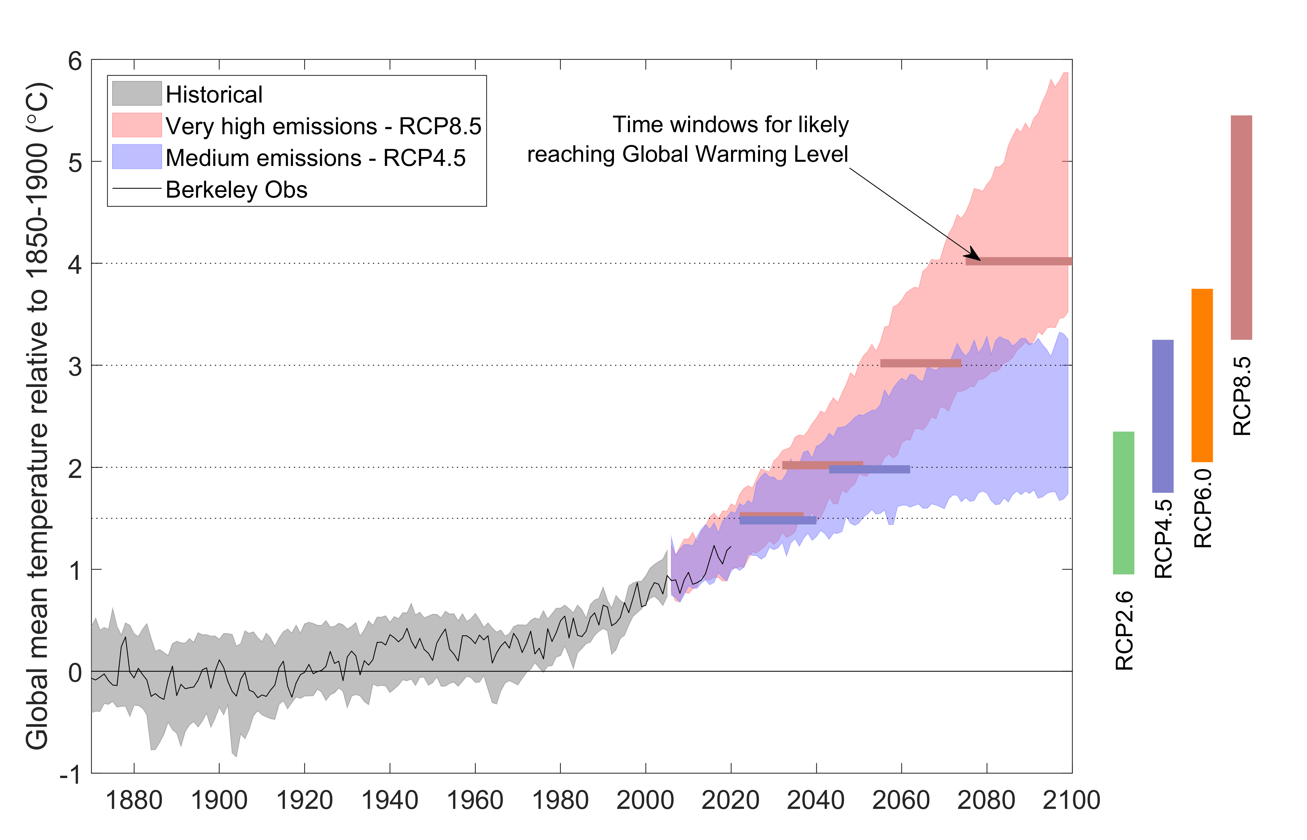
Figure 3 Comparison of speed of warming for different climate scenarios. (Source: Adapted from IPCC 2013)
Up to the year 2040, there is not much difference between the greenhouse gas concentrations and global warming estimates for the different RCPs; for example, RCP2.6 is similar to RCP4.5 and close to RCP8.5 even out to 2050. Beyond 2050, the concentrations and global warming estimates strongly diverge, and the ranges of likely global warming also start to separate (Figure 2). Figure 3 indicates that during the mid part of the century, the global warming occuring under RCP2.6 can be thought of as occuring a decade or two later than under RCP8.5, before plateauing by around 2050–2060. If detailed projection for RCP2.6 is required, then the rule of thumb can be applied of using RCP4.5 to 2040–2060 and then making the assumption that the climate plateaus at that warming for the rest of the century (the outputs from RCP8.5 for mid-century are not appropriate, as they are already starting to diverge).
The ESCI project recommends scenario analysis using RCP4.5 and RCP8.5 for physical risk assessments, but if RCP2.6 is required, a more detailed discussion of scaling data for an RCP2.6 pathway is given in ESCI Key Concept—Scaling data for RCP2.6 (and other pathways).
References
Hausfather Z and Peters GP (2020) Emissions—the ‘business as usual’ story is misleading. Nature 577:618–20 https://doi.org/10.1038/d41586-020-00177-3
IPCC (2013). ‘Summary for Policymakers’ in Climate Change 2013: The Physical Science Basis. Contribution of Working Group I to the Fifth Assessment Report of the Intergovernmental Panel on Climate Change (eds TF Stocker, D Qin, G-K Plattner et al. Cambridge: Cambridge University Press).
IPCC (2019). Special Report on the Ocean and Cryosphere in a Changing Climate . (ipcc.ch)
Schwalm CR, Glendon S, Duffy PB (2020). ‘RCP8.5 tracks cumulative CO2 emissions’ Proceedings of the National Academy of Sciences of the United States of America 17(33):19656–57.
van Vuuren DP, Edmonds J, Kainuma M, et al. (2011). ‘The representative concentration pathways: an overview’ Climatic Change 109:5–31
Notes
1 Disaster Risk Handbook 04 – Climate and disaster risks: Guidance on Scenarios
2 Most of this text is taken from the Coast Adapt website where you can find more detail on societal changes that would be required for each pathway.
3 Task Force on Climate-related Financial Disclosure
4 Note, this is no longer appropriately called ‘business as usual’ (Hausfather and Peters 2020).
5 Climate change transition risk could include policy change which requires pricing in of greenhouse gas emissions, unforeseen changes in customer behaviour, reputational or legal risk as a result of increasing stakeholder concern or negative stakeholder feedback, or technology risk if transition to new technology occurs earlier than forecast. See for example: http://et-risk.eu/wp-content/uploads/2018/02/Investor-primer-to-transition-risk-analysis.pdf
6 See ESCI Key Concepts —Scaling data for RCP2.6 (and other uses).
Downloads
DownloadAll figures (zip 901.9 KB)
Climate Models and Downscaling
- Climate Models
- Dynamical Downscaling
- Statistical Downscaling
- Delta-Scaling Historical Data
- Quantile-Matching Model-Simulated Data
- Caveats
- References
- Downloads
Climate models
Global climate models (GCMs) represent weather and climate processes mathematically over a three-dimensional grid of points across the globe, including the surface, oceans, cryosphere and atmosphere (Figure 1). These models can be driven by changes in the Earth's energy balance caused by natural factors (e.g. volcanic eruptions, changes in the Earth’s orbit) or anthropogenic factors (e.g. greenhouse gas increases, land-use change). Calculations are made for hundreds of climate variables, at sub-hourly time steps, over thousands of grid points, over hundreds of years, which requires the use of super-computers and significant data storage. Climate models help us understand interactions between processes within the climate system, including drivers of past climate change, as well as how the climate may change in future based on emission scenarios for greenhouse gases and aerosols.
High-quality observations are required to assess climate model performance. There are several standard performance metrics and regionally specific metrics (CSIRO and BoM 2015). These metrics and expert judgements are used to determine which models perform well enough for use in risk assessments.
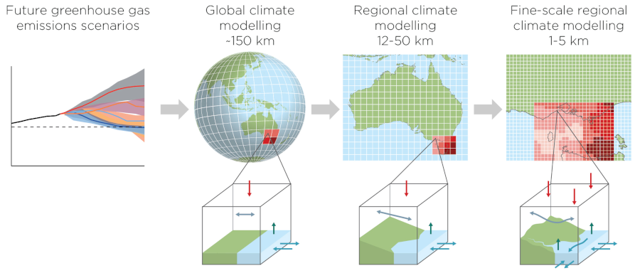
Figure 1. Schematic representation of the downscaling process.
A key limitation of global climate models is coarse spatial resolution. Even with the most powerful supercomputers, the spacing of grid points is typically 100–150 km. This means it can be hard to include the influence of surface features (e.g. mountains, coastlines and vegetation) on weather and climate. It also means that global climate models do a poor job of modelling weather and climate processes, such as thunderstorms, operating on smaller scales. To address these limitations, various downscaling techniques are used, each of which has strengths and weaknesses (Table 1).
Dynamical downscaling
Dynamical downscaling involves using a high-resolution regional climate model (RCM) within a global model These RCMs can capture regional phenomena missing from global climate models but they still require parameterizations to estimate the role of climate processes that occur on smaller scales. RCMs are driven at their lateral boundaries by information from a global climate model so the RCM will inherit biases in the broad-scale climate simulated by the global model (Ekstrom and and Grose 2014; Rummukainen 2015). The added value of downscaling is evident across the majority of Australia (Figure 1) and shows where plausible improvements in future climate projections are conferred by RCMs (Di Virgilio et al. 2020).
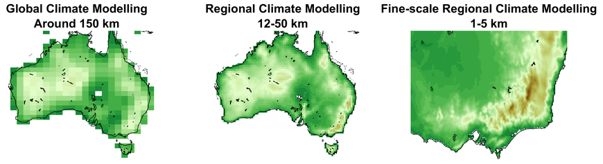
Figure 2. Added value from downscaling with the effect of topography shown for projected change in total rainfall in the Australian Alps between 1990–2009 and 2060–2079 under RCP8.5 in Winter (June, July August). Projections use 6 CMIP5 models (left-hand plot) then downscaled with CCAM-5 (right-hand plot). Scale gives percent change. (Source: Grose et al. 2019)
ESCI has provided dynamical downscaling based on multiple RCMs, namely the BARPA model (Bureau of Meteorology Atmospheric high-resolution Regional Projections for Australia) as well as CCAM (Conformal Cubic Atmospheric Model) projections. ESCI also used also included the new NARCliM (NSW and ACT Regional Climate Modelling) projections. (Quantile matching for extremes (QME) calibration has also been applied to the ESCI dynamically downscaled data sets so that they are ‘application ready’, QME is discussed later in this document.)
Performing these simulations has a high computational cost. This limits the number of global climate models that can be downscaled so it is important to select a subset of global climate models that (a) perform well and (b) represent the range of projected changes simulated by the full set of global climate models. Climate projections based on RCMs exist for most land regions of the world including Australia through the Coordinated Regional Downscaling (CORDEX) project. Dynamical downscaling of CMIP51 global climate models is available for Australia (CSIRO and BoM 2015), as well as in Victoria (Victorian Government 2019), South Australia (SAE 2019) and Queensland (Queensland Longpaddock 2019). Dynamical downscaling of older CMIP3 GCMs is available for Tasmania (ACE CRC 2010), south-eastern Australia (SEACI 2012), south-western Australia (Andrys et al. 2017), New South Wales and the Australian Capital Territory (NARCliM, 2020). The ESCI project is the first time that a set of multiple regional climate models have been used to provide nationally consistent data sets.
Statistical downscaling
Statistical downscaling involves the use of statistical methods to (1) adjust historical weather data to represent future weather data (e.g. delta-scaling or quantile-scaling of historical data) or (2) adjust model-simulated data to improve representation of historical and future weather and climate data (e.g. using quantile-matching trained on observations). Statistical downscaling for the whole of Australia is available for CMIP3 (Queensland Government 2020) and CMIP5 GCMs (CSIRO and BoM 2015; SimClim 2020). Statistical downscaling from CMIP5 GCMs is available for South Australia (Charles and Fu 2015) and from CMIP3 GCMs for Western Australia (IOCI 2012).
Delta-scaling historical data
Delta-scaling is very simple. The monthly-mean changes in a given climate variable, simulated by a climate model, are applied to observed data. For example, the simulated change in January mean temperature by 2050 is added to 30 years of historical January daily temperature data to create daily January temperature data for 30 years centred on 2050.
Hence, the future daily data have the same sequence of weather events as in historical daily data, with an adjustment. It assumes no change in variance, so extreme events change by the same amount as the mean climate, which may be too simplistic. This is where quantile-matching of model-simulated data may help.
Method | Strengths | Weaknesses |
|---|---|---|
Trend extrapolation |
|
|
Delta scaling of observations using GCM output |
|
|
Quantile scaling of observations using GCM output |
|
|
Statistical downscaling of GCM outputs |
|
|
Dynamical downscaling using RCMs with bias correction |
|
|
Quantile-matching model-simulated data
Quantile-scaling methods scale different parts of a climate variable's frequency distribution at different rates. The quantile-scaling factors are calculated from a climate model simulation, for example the 1st percentile may increase by 1.2 oC, 2nd percentile by 1.3 oC, . . ., 10th percentile by 1.6 oC, . . ., 90th percentile by 2.0 oC, 99th percentile by 2.2 oC. Each of these scaling factors would then be applied to the equivalent percentiles in historical data to create a future data set. Again, the future daily data cover the same sequence of weather events as in historical daily data, with an adjustment, allowing for projected changes in variance.2
The same approach can be used to correct biases in the climate models. While climate models continue to improve, the simulation of current climate features is imperfect to some degree (e.g. too hot/cold/wet/dry), and global model climate models were inItiated at a (historical) point in time so they will not match present-day observations. If the biases are large the simulation would be considered unsuitable for impact assessments. If the biases are reasonably small and systematic, various statistical techniques can be used to adjust a simulated climate variable toward historical values. These adjustments can then also be applied to a future climate simulation, giving a bias-adjusted climate projection. Some methods can preserve simulated changes in the intensity, frequency and duration of weather events.
‘Quantile-matching for extremes’ (QME: Dowdy 2020) is a sophisticated technique tailored specifically for extremes that has been used in the ESCI project to produce calibrated projections data. These projections with QME applied are the primary data sets recommended for many variables from this ESCI project, including for daily values of temperature and derived quantities such as FFDI, as well as for extremes such as ARI values.
Caveats
Climate models have limitations and uncertainties at regional and local scales over the next decade are strongly influenced by natural variability, which is hard to predict. Observed climate trends over recent decades may be the best choice to inform climate trends over the next decade.
The ESCI project recommends downscaled data sets for use for climate risk assessments over the next two decades and beyond. These can provide high-resolution climate projections which account for topographic features and other physical effects. However, downscaled simulations may include regional errors, especially at the weather scale. The numerical precision of these data must not be confused with accuracy. The downscaled projections should be considered plausible, rather than precise, based on the best available information.
Where possible, uncertainties have been estimated and confidence ratings have been provided,3 and these, and the caveats above, should be included in risk assessment documentation.
Data from a new set of CMIP6 GCMs are currently being evaluated.4 Some of these GCMs will eventually be downscaled in the CORDEX-2 experiment. Over the coming decade, it is hoped that a paradigm shift in GCMs will enable simulations much finer resolution, avoiding the need for downscaling. Therefore, improved data sets are in the pipeline.
References
ACE CRC (2010). Climate Futures for Tasmania
Andrys J, Kala J, and Lyons TJ (2017). ‘Regional climate projections of mean and extreme climate for the southwest of Western Australia (1970–1999 compared to 2030–2059)’ Climate Dynamics 48(5–6):1723–47. https://doi.org/10.1007/s00382-016-3169-5
Charles SP and Fu G (2015). Statistically Downscaled Climate Change Projections for South Australia. Goyder Institute for Water Research, Technical Report Series No. 15/1. http://www.goyderinstitute.org/_r91/media/system/attrib/file/82/CC%20Task%203%20CSIRO%20Final%20Report_web.pdf
Di Virgilio G, Evans JP, Di Luca A, et al. (2020). ‘Realised added value in dynamical downscaling of Australian climate change’ Climate Dynamics 54:4675–92
Dowdy AJ (2020). ‘Seamless climate change projections and seasonal predictions for bushfires in Australia’ Journal of Southern Hemisphere Earth Systems Science 70(1):20–38 https://doi.org/10.1071/ES20001
Ekstrom M, Grose M, and Whetton P (2014). ‘An appraisal of downscaling methods used in climate change research’ WIREs Climate Change https://doi.org/10.1002/wcc.339
Grose M, Sykktus J, Thatcher M, et al. (2019). ‘The role of topography on projected rainfall change in mid-latitude mountain regions’ Climate Dynamics https://doi.org/10.1007/s00382-019-04736-x
Hennessy K, Webb L, and Clarke J. ‘Using climate change data in impact assessment and adaptation planning’ Chapter 9 in Climate Change in Australia Technical Report. www.climatechangeinaustralia.gov.au
IOCI (2012). Western Australia’s weather and climate. A synthesis of Indian Ocean Climate Initiative Stage 3 research. http://www.ioci.org.au/publications/ioci-stage-3/cat_view/17-ioci-stage-3/23-reports.html
NARCliM (2019). http://www.ccrc.unsw.edu.au/NARCliM/
Queensland Government (2019). Consistent Climate Scenarios. https://data.qld.gov.au/dataset/consistent-climate-scenarios
Queensland Longpaddock (2019). Queensland Future Climate
Rummukainen M. Added value in regional climate modeling’ (2015) WIREs Climate Change https://doi.org/10.1002/wcc.378
SEACI (2012). http://www.seaci.org
SimClim (2019). http://www.climsystems.com
Victorian Government (2019) Victorian Climate Projections 2019. Victorian Climate Projections 2019 climatechange.vic.gov.au
WA Agriculture (2019). https://www.agric.wa.gov.au/climate-change/climate-projections-western-australia
Wilby RL, Troni J, Biot Y, et al. ‘A review of climate risk information for adaptation and development planning’ (2009) International Journal of Climatology https://doi.org/10.1002/joc.1839
Notes
1 CMIP refers to models evaluated by the Intergovernmental Panel in Climate Change IPCC Coupled Model Inter-comparison Projects. These are numbered to align with IPCC assessment reports, thus CMIP5 (CMIP5) was published with Assessment Report 5 (AR5) in 2014. CMIP6 models are expected to be released with AR6 in 2021. See ESCI Key Concepts —CMIP6 models.
2 ESCI Case study—Temperature trends and demand uses the quantile-scaling method to adjust historical half-hourly temperatures by projected daily temperatures in order to produce a projection with the same statistical properties as observations.
3 See Key Concepts —Climate projection confidence and uncertainty.
4 See Key Concepts —New data sets available from CMIP6
Downloads
DownloadAll figures (zip 693.9 KB)
Climate Projection Confidence and Uncertainty
- Introduction
- Confidence
- Uncertainty
- Sampling uncertainty in practice
- Climate projections
- References
- Downloads
Introduction
The ESCI project is providing climate projections and data to support the Australian electricity sector assess physical risk over the next 80 years. However, it is important to note that climate projections have different levels of confidence and uncertainty. Scientists analyse evidence from a range of credible sources to estimate confidence and uncertainty. The Intergovernmental Panel on Climate Change (IPCC) provides ‘best practice’ guidance on how to assess confidence and uncertainty (Mastrandrea et al. 2011).
Confidence
Confidence in a climate projection is based on the type, amount, quality and consistency of evidence (e.g. process understanding, theory, data, expert judgment) and the degree of agreement between different lines of evidence. Confidence is expressed qualitatively (i.e. very low, low, medium, high and very high). For example, where there is limited evidence with low agreement, confidence is low, but where evidence is robust with high agreement, confidence is high.
Lines of evidence have been collected and documented in tables [Lines of Evidence technical report report]. This information includes analysis of long-term observed trends, the range of results from global climate model simulations of future climate, uncertainties relating to a modelling approach’s ability to simulate physical processes and observed features (such as the seasonal cycle or spatial detail of extremes), as well as the influence of large-scale drivers (e.g. the El Niño Southern Oscillation) in the historical and future climates.
Hazard | Confidence |
|---|---|
Increases in average and extreme temperature | Very high |
Decreases in winter and spring rainfall in Southern Australia | High |
Winter rainfall decreases in the east | Medium |
Increase in extreme daily rainfall | Medium |
Increases in extreme fire weather days | High confidence except in the east where there is medium confidence |
Decreases in the number of east coast lows | Medium |
Increases in severe windspeeds | Low |
Uncertainty
Uncertainty is expressed
quantitatively by presenting a probability distribution or a percentile
range within that distribution (e.g. 10th–90th percentile range). In
addition to the uncertainty range, it is useful to provide a central
estimate (e.g. the average or median).
The three main sources of uncertainty in climate projections are:
- Natural climate variability including fluctuations in daily weather, seasonal/annual climate (e.g. El Niño Southern Oscillation) and decadal climate (e.g. Pacific Decadal Oscillation).
- How greenhouse gas and aerosol concentrations may change in response to socio-economic change, technological change, energy transitions, and land-use change. This is described using 'pathways' (see Key Concept A: Representative emissions pathways ). The ESCI project provides data for a low concentration pathway (RCP4.5—leading to lower global warming) and a high concentration pathway (RCP8.5—leading to higher global warming).
- How regional weather and climate respond to changing greenhouse gases and aerosols. This information is derived from climate models, each of which provides a different simulation of future weather and climate at a given location. The ESCI standard data set is based on simulations from seven climate models that (i) perform well in the Australian region and (ii) sample most of the range of projected changes in temperature, rainfall, windspeed and fire weather from 40 climate models.
Natural climate variability contributes the largest proportion of uncertainty over the next decade. Regional climate modelling contributes a significant proportion of uncertainty from 2030–2050. In the longer term, uncertainty is dominated by different greenhouse gas and aerosol concentration pathways (Figure 1).
.")
Figure 1 Proportion of climate projection uncertainty due to different factors over the 21st century (CSIRO and BoM 2015).
Greenhouse gas concentration pathways are similar up to about the year 2040, then diverge after 2050 (Figure 2). Therefore, the choice of pathway becomes more important after 2050. Simulations from climate models driven by these pathways show that global warming estimates are similar up to about 2040 then diverge (Figure 3). By the year 2100, the global warming is about 1.0 °C for RCP2.6 and about 4.0 °C for RCP8.5.
. (Source: van Vuuren et al. 2011)")
Figure 2 Representative concentration pathways for carbon dioxide (CO2). (Source: van Vuuren et al. 2011)
The regional climate response simulated by climate models can be visualised in a variety of ways, including maps, time series and bar charts. The Climate Change in Australia website provides examples for selected regions, seasons, concentration pathways and future years. Examples are shown in Figures 4–7 for temperature and rainfall.
Sampling uncertainty in practice
The three sources of uncertainty have been sampled by the ESCI project. There are two options:
- Using the ESCI minimum standard data set: historical weather and climate data from the Bureau of Meteorology plus future weather and climate data. Data are available from four climate model simulations for RCP4.5 and RCP8.5 for daily, monthly and annual temperature, rainfall, windspeed and fire weather. Future weather and climate data have been bias-adjusted to improve consistency with historical data.
- Using an alternative ESCI data set: provides sub-daily (e.g. hourly) data for a broader range of climate variables from 16 climate model simulations for RCP4.5 and RCP8.5. This data set is much larger and has not been bias-adjusted so advice should be sought from climate scientists if the data are used in risk assessments to inform investment decisions.
 and RCP8.5 (from 39 climate models), relative to 1986–2005. (Source: IPCC 2013)")
Figure 3 Historical and future global warming. Projections are based on RCP4.5 (from 32 climate models) and RCP8.5 (from 39 climate models), relative to 1986–2005. (Source: IPCC 2013)
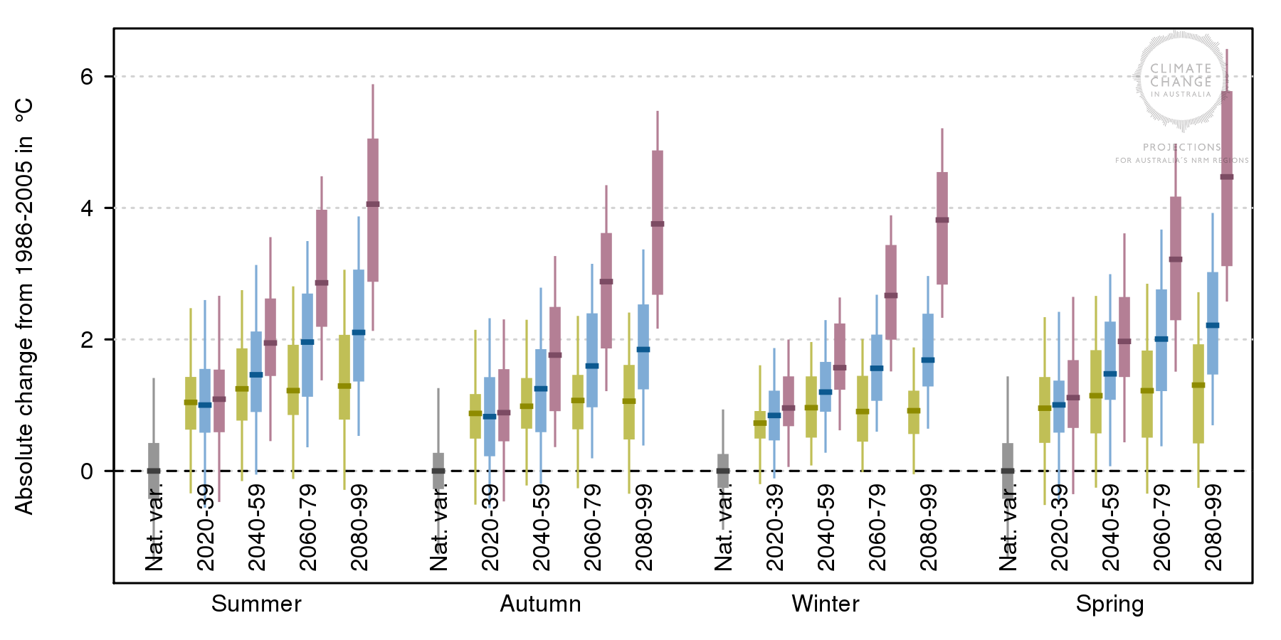
Figure 4. Maximum temperature projections for the Murray Basin. Changes are given in % relative to 1986–2005 under RCP2.6 (green), RCP4.5 (blue) and RCP8.5 (purple). Natural climate variability is represented by the grey bar. The middle (bold) line is the median value of the model simulations (20-year moving average climate); half the model results fall above and half below this line. The bars show the range (10th–90th percentile) of model simulations of 20-year average climate. Line segments represent the projected range (10th–90th percentile) of individual years taking into account year-to-year variability in addition to the long-term response (20-year average). (Source: Climate Change in Australia )
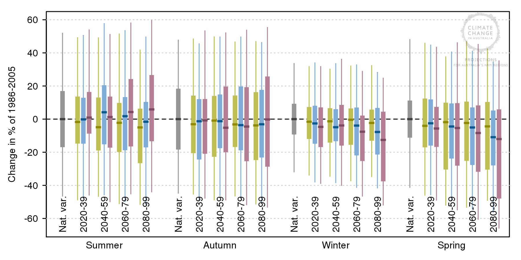
Figure 5 Rainfall projections for the Murray Basin. Changes are given in % relative to 1986–2005 under RCP2.6 (green), RCP4.5 (blue) and RCP8.5 (purple). Natural climate variability is represented by the grey bar. The middle (bold) line is the median value of the model simulations (20-year moving average climate); half the model results fall above and half below this line. The bars show the range (10th–90th percentile) of model simulations of 20-year average climate. Line segments represent the projected range (10th–90th percentile) of individual years taking into account year-to-year variability in addition to the long-term response (20-year average). (Source: Climate Change in Australia )
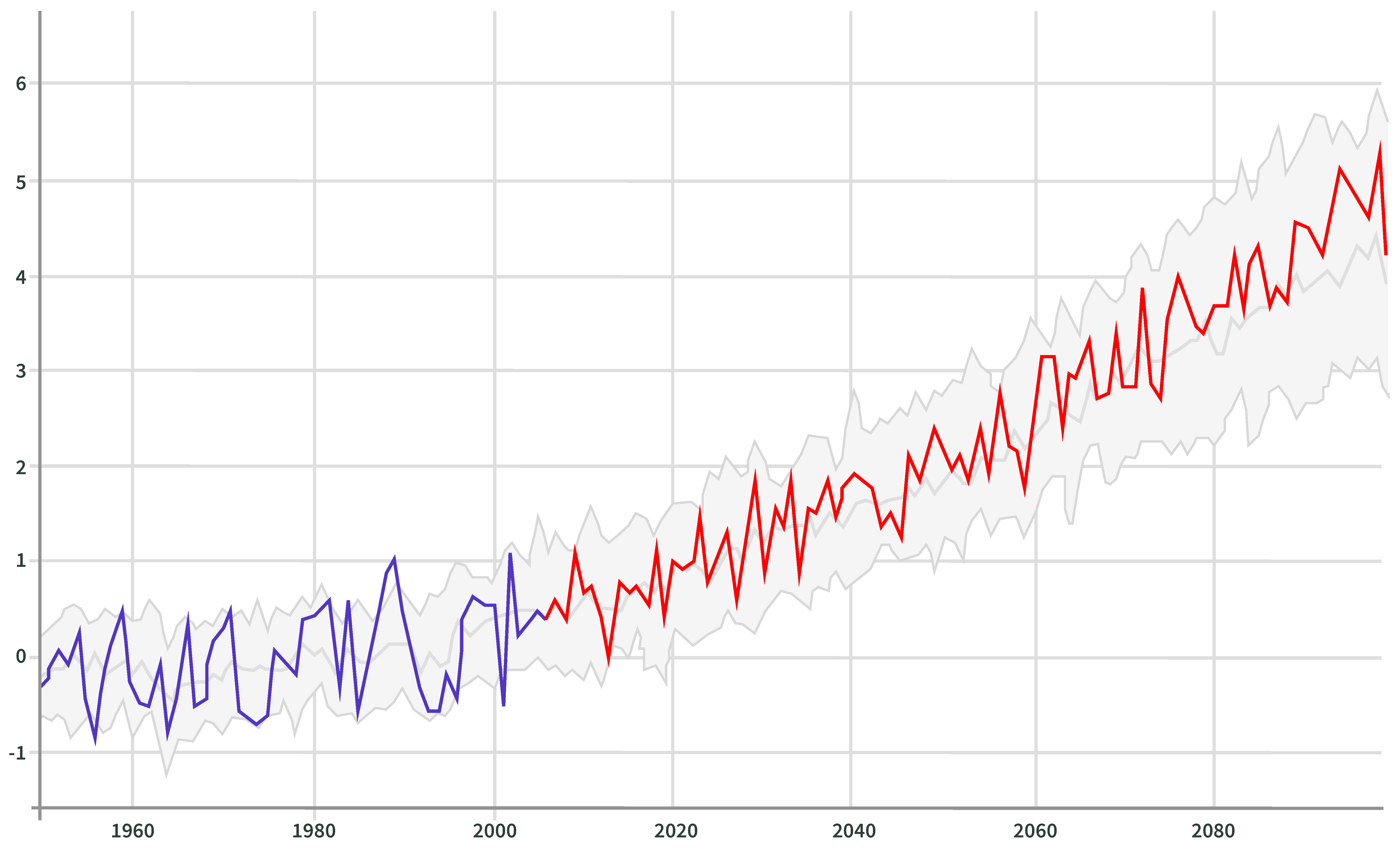
Figure 6 Twenty-year running-average temperature projection timeseries for the Murray Basin for RCP8.5. The grey-shaded area shows the 10th–90th percentile range of uncertainty from 40 climate models, and the central grey line is the median. Historical data (blue) and ACCESS1.0 climate model data (red) are superimposed. (Source: Climate Change in Australia )
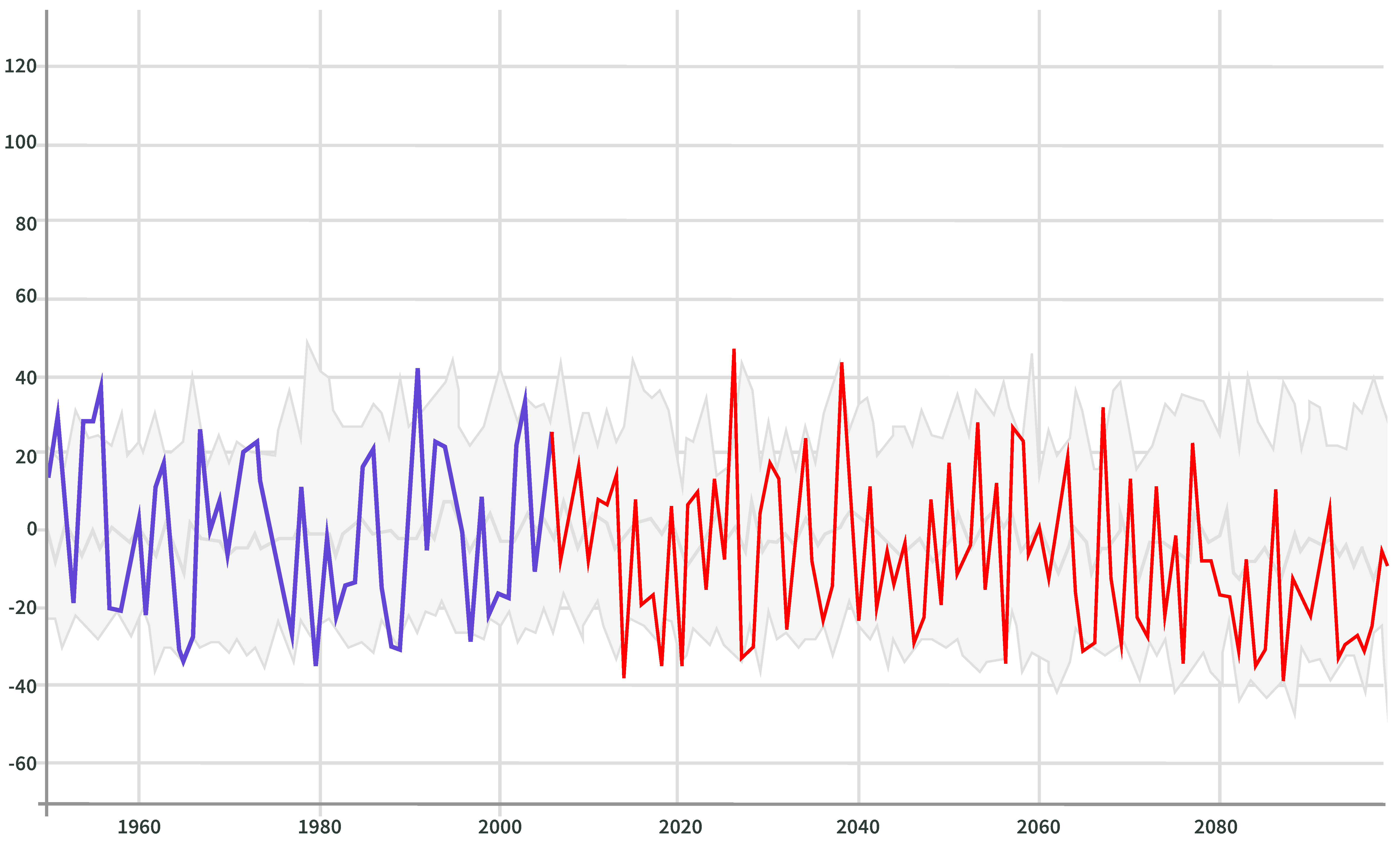
Figure 7 Twenty-year running-average rainfall projection timeseries for the Murray Basin for RCP8.5. The grey-shaded area shows the 10th–90th percentile range of uncertainty from 40 climate models, and the central grey line is the median. Historical data (blue) and ACCESS1.0 climate model data (red) are superimposed. (Source: Climate Change in Australia )
Climate projections
Climate projections are derived from climate models that have limitations. Uncertainties at regional and local scales over the next decade are strongly influenced by natural variability, which is hard to predict. Observed climate trends over recent decades can inform future climate trends over the next decade. The CMIP5 global climate models (GCMs) have coarse-resolution (about 100–150 km between data points) and provide useful information projections over the next two decades and beyond at global and continental scales. Some GCMs include regional errors, so we have selected a subset of GCMs that perform well in the Australian region. Nevertheless, GCMs cannot adequately represent weather-scale (1–10 km) phenomena, so downscaling methods have been used. Dynamical downscaling simulates important climate processes at finer scales (10–50 km) and this tends to improve the simulation of regional climate variability and change. However, downscaled simulations may include regional errors, especially at the weather scale. Statistical downscaling has been used to reduce these errors and provide daily data on a 5 km grid. The numerical precision of these data must not be confused with accuracy. The downscaled projections should be considered indicative, rather than precise, based on the best available information. Where possible, uncertainties have been estimated and confidence ratings have been provided.
Data from a new set of CMIP6 GCMs is currently being evaluated. Some of these GCMs will eventually be downscaled in the CORDEX-2 experiment. Over the coming decade, it is hoped that a paradigm shift in climate science and computer technology will enable simulations with much finer resolution, avoiding the need for downscaling.
| Climate variable | Observed trend | Change by 2030 | Change by 2050 | Change by 2080 | Confidence rating | Source |
|---|---|---|---|---|---|---|
Annual average temperature | +1.4 °C from 1910 to 2019 | +0.6 to 1.4 °C | +0.5 to 1.5 °C +1.5 to 2.5 °C | +0.5 to 1.5 °C
+2.5 to 5.0 °C | Very high | NESP ESCC Hub (2020) |
Annual average rainfall | Northern Australian rainfall has increased since the 1970s, while April–October rainfall has decreased 16% since the 1970s in south-western Australia and 12% since the late 1990s in south-eastern Australia | East: –13 to +5% North: –9 to +4% South: –9 to +2 % Rangelands: –10 to +6 % | East: –13 to +7% (RCP2.6), -17 to +8% (RCP8.5) North: -12 to +5% (RCP2.6), -8 to +11% (RCP8.5) South: –15 to +2 % (RCP2.6), –14 to +3% (RCP8.5) Rangelands: –18 to +3 % (RCP2.6), –15 to +8% (RCP8.5) | East: –16 to +6% (RCP2.6), –25 to +12% (RCP8.5) North: –12 to +3% (RCP2.6), –26 to +23% (RCP8.5) South: –15 to +3 % (RCP2.6), –26 to +4% (RCP8.5) Rangelands: –21 to +3 % (RCP2.6), –32 to +18% (RCP8.5) | High: winter-spring decrease in south Medium: winter decrease in east Low: other regions and seasons | BoM and CSIRO (2020) NESP ESCC Hub (2020) |
Annual number of days > 35 °C | Increased from 1910–2019 | +20 to +70% | N/A | +25 to +85% (RCP2.6) +80 to +350% (RCP8.5) | Very high | CCiA (2015) ESCI 2021 |
Extreme windspeed | Uncertain | Increase in south and east | Increase in south and east | East: –56 to +33% (median +8%) (RCP8.5) South: –49 to +45% (median +7%) (RCP8.5) | Low | ESCI (2021) |
Number of East Coast Lows | –10% from 1986–2019 | –15 to –5% | –15 to –5% (RCP2.6), –30 to –10% (RCP8.5) | –15 to –5% (RCP2.6), –50 to –20% (RCP8.5 | Medium | NESP ESCC Hub (2020) ESCI (2021) |
Annual number of extreme fire weather days (> 90th percentile) | Increased since the 1950s, especially in southern Australia. | East: 0 to +30% Elsewhere: +5 to +35% | East: 0 to +30% (RCP2.6), 0 to +60% (RCP8.5) Elsewhere: +5 to +35% (RCP2.6), +10 to +70% (RCP8.5) | East: 0 to +30% (RCP2.6), 0 to +110% (RCP8.5) +5 to +35% (RCP2.6), +20 to +130% (RCP8.5) | Medium: east coast High: elsewhere | BoM & CSIRO (2021) NESP ESCC Hub (2020) |
References
BoM and CSIRO (2020). State of the Climate
CSIRO and BoM (2015). Climate Change in Australia Technical Report
ESCI (2021). Standardised Method for Projections Likelihood: WPC Technical Report for the ESCI project.
IPCC. ‘Summary for Policymakers’ in Climate Change 2013: The Physical Science Basis. Contribution of Working Group I to the Fifth Assessment Report of the Intergovernmental Panel on Climate Change. (Cambridge: Cambridge University Press, 2013).
Mastrandrea MD, Mach KJ, Plattner G-K et al. ‘The IPCC AR5 guidance note on consistent treatment of uncertainties: a common approach across the working groups’ (2011) 108 Climatic Change 675–91. https://doi.org/10.1007/s10584-011-0178-6
NESP ESCC Hub (2020). Scenario Analysis of Climate-Related Physical Risk for Buildings and Infrastructure: Climate Science Guidance. Technical report by the National Environmental Science Program (NESP) Earth Systems and Climate Change Science (ESCC) Hub for the Climate Measurement Standards Initiative , ESCC Hub Report No. 21.
van Vuuren DP, Edmonds J, Kainuma M et al. ‘The representative concentration pathways: an overview’ (2011) 109 Climatic Change 5–31. https://doi.org/10.1007/s10584-011-0148-z
Downloads
DownloadAll figures (zip 1.1 MB)
Deriving Average Recurrence Interval (ARI) Maps
- Summary
- ARI for an Ensemble of Models
- ARI for Individual Climate Model Simulations
- Sample Maps of ARI-10 Outputs
- Downloads
Summary
The Average Recurrence Interval (ARI) is the threshold value of a variable that is expected to be exceeded, on average, once in a certain number of years (the ‘return period’). These ARI values are based on the most extreme values observed through a given period, spanning a minimum of 20 years. For example, the ARI-10 of daily maximum temperature represents the daily temperature value that would be expected to be exceeded on average once every 10 years, based on the period analysed.
The ARI in years can alternatively be described using probabilities, and are sometimes/interchangeably described as an Average Exceedance Probability (AEP) or Probability of Exceedance (POE). These represent the likelihood of an event of that magnitude being exceeded in a given year. The probabilities are approximately inversely proportional to the ARI in years; in the above example, an ARI-20 (1-in-20 year event) represents the likelihood of a daily value exceeding this number in a given year. So it is 1-in-20 years, which is 1/20 = 0.05 = 5% POE or AEP.
Thresholds such as the ARI-10 of daily maximum temperatures are used in numerous existing forecasting, planning and asset management decision-making processes in the sector. As the climate changes, the values of such thresholds are projected to change, requiring consideration by electricity sector decision-makers.
ARI for an ensemble of models
While climate models project increases in temperature with a high level of agreement and confidence, regional impacts vary and there is increased uncertainty at finer spatial resolution. Following best practice in climate risk analysis, a large ensemble of climate models has been collated to explore the uncertainty in regional impacts by comparing different results from different climate models. Given that extremes are, by definition, rare events, the 10th, 50th and 90th percentiles for the ensemble were calculated using a method of statistical modelling called the Generalised Extreme Value distribution (GEV), which involves fitting a parametric curve to the extremes of the data set. In this method the series of annual maximum values (or, in the case of coldest temperatures, minimum values) from the time period of the data are used to fit the parameters of the GEV distribution using the L-moments method. The parameters from the GEV analysis are then used to derive the values expected once in N years for each variable. The ESCI project uses a baseline of 1986–2005; the simulated changes in ARI-10 daily maximum temperature was calculated relative to this baseline. The time periods consisted of 20-year blocks, considered to be the minimum requirement to obtain a reasonable fit to the data while minimising the impact of long-term trends in the input data.
Using an ensemble of multiple models reduces the uncertainties around natural variability during a 20-year period compared with considering a single model. This increased stability makes ensemble projections for ARI a useful tool for looking at single variable extremes, however, the ensemble approach means that it cannot be used for simultaneously comparing multi-variable extremes, as the values of the different variables at each grid point may come from different models and are therefore not directly comparable.1 This is because combining variable from different models is not internally consistent and may not be climatologically plausible.
Values of ARI for several return periods (ARI-2, ARI-5, ARI-10 and ARI-20) have been generated using ensembles for a number of key climate variables, including daily maximum temperature and daily Forest Fire Danger Index (FFDI).
The ensemble analysis was derived for a variety of global climate model products,2 and from the Australian Gridded Climate Data (AGCD) from the Australian Bureau of Meteorology, which provide spatially interpolated historical climate information on a 0.05 degree grid.
ARI for individual climate model simulations
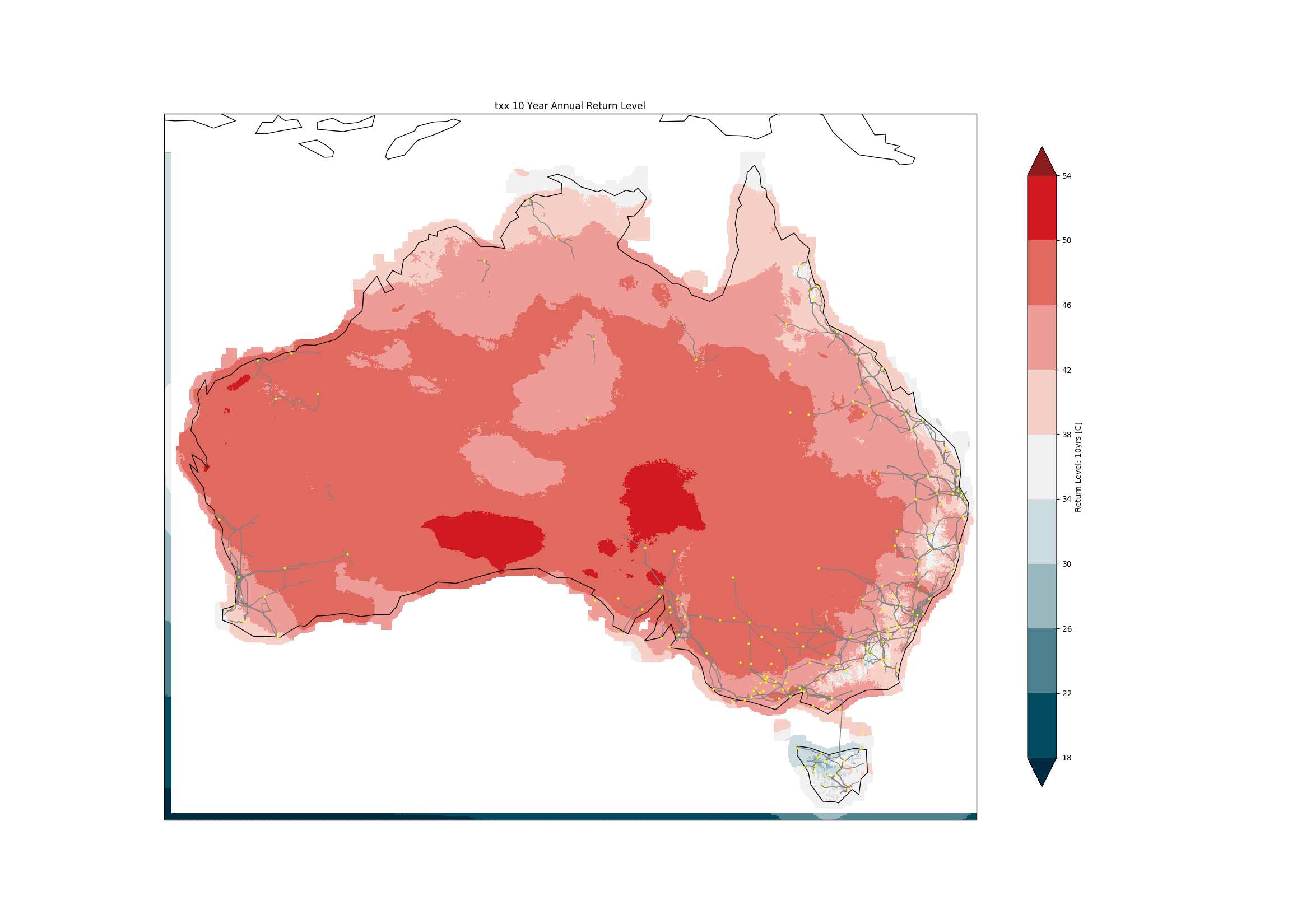
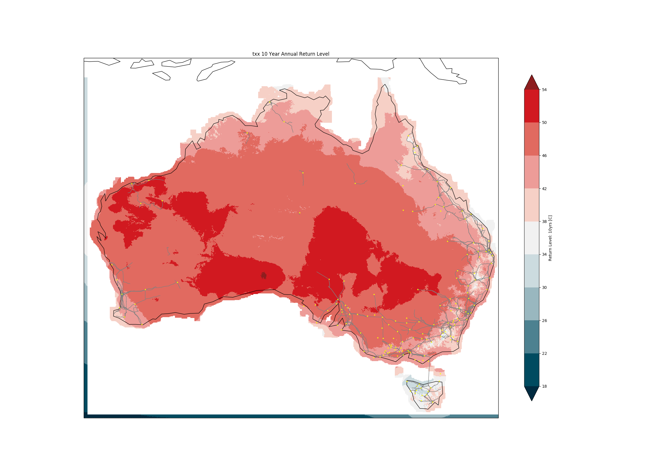
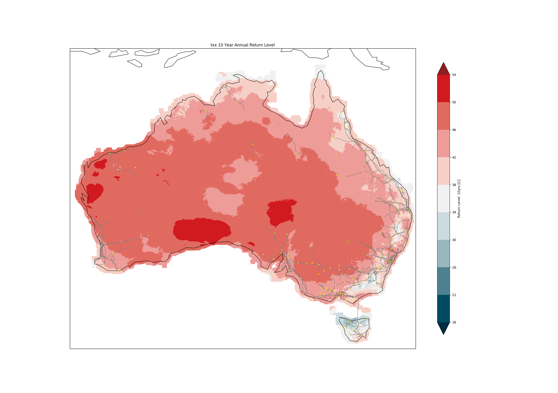
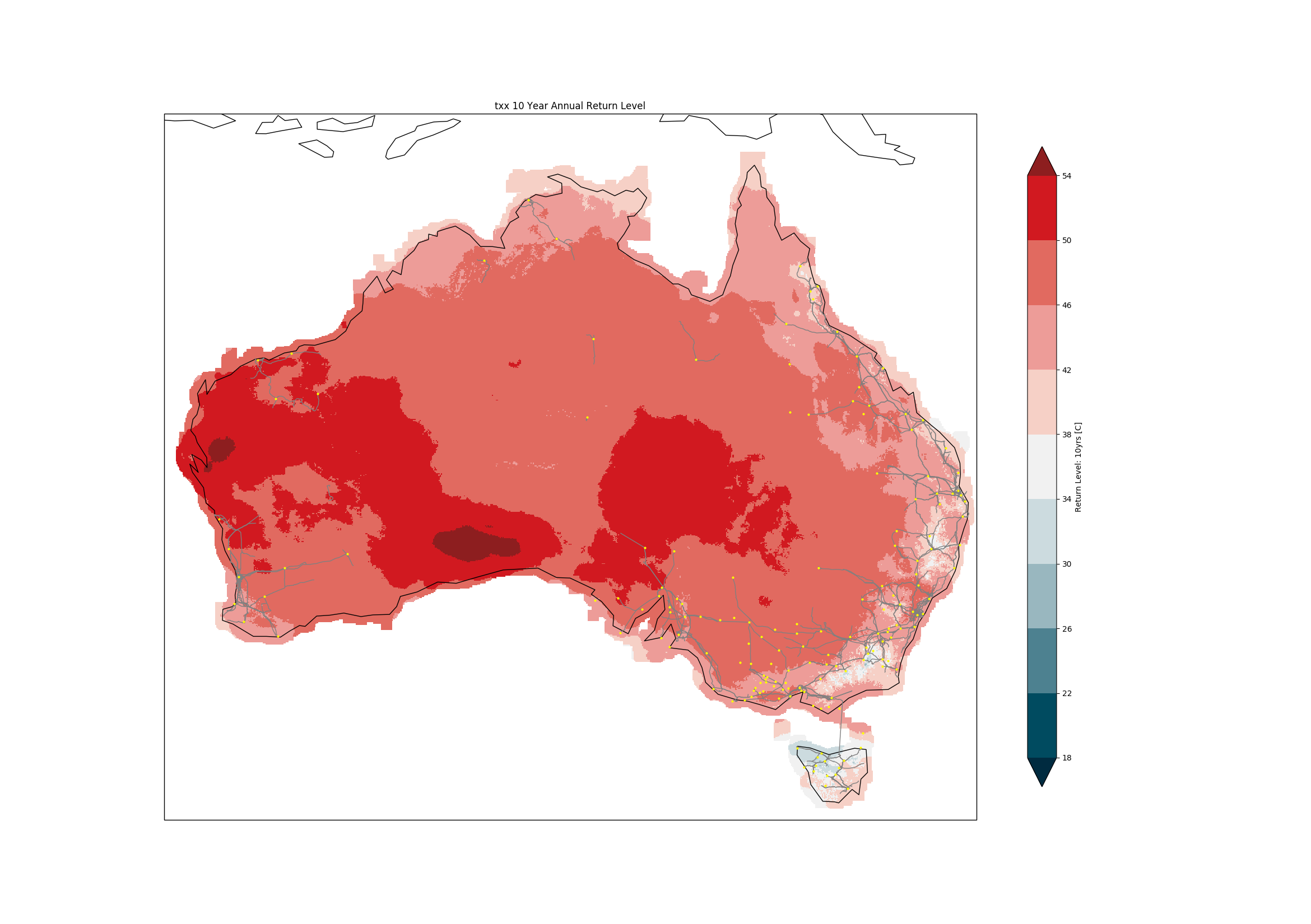
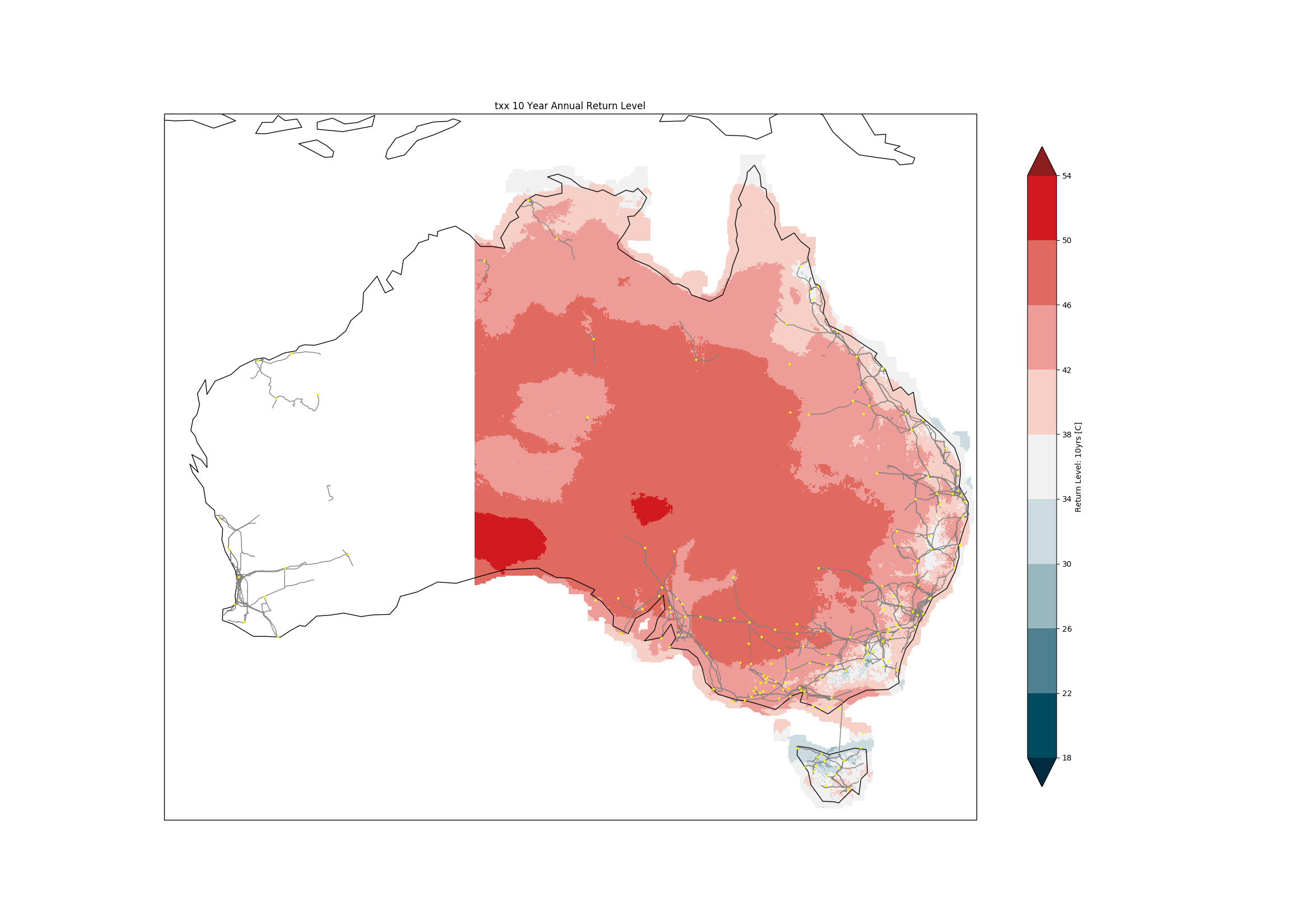
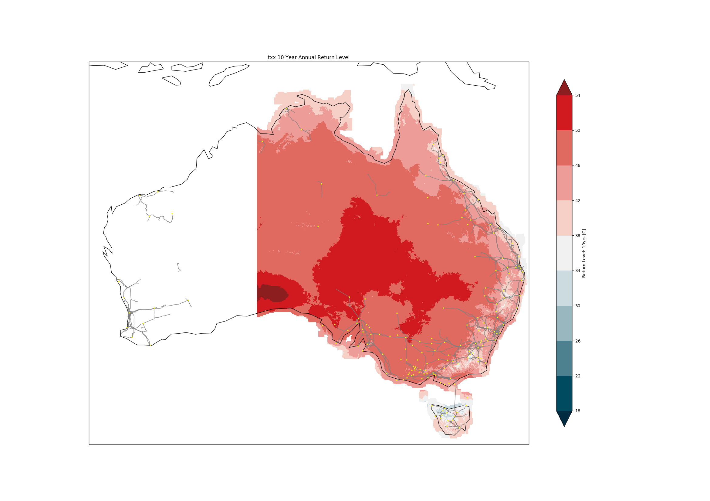
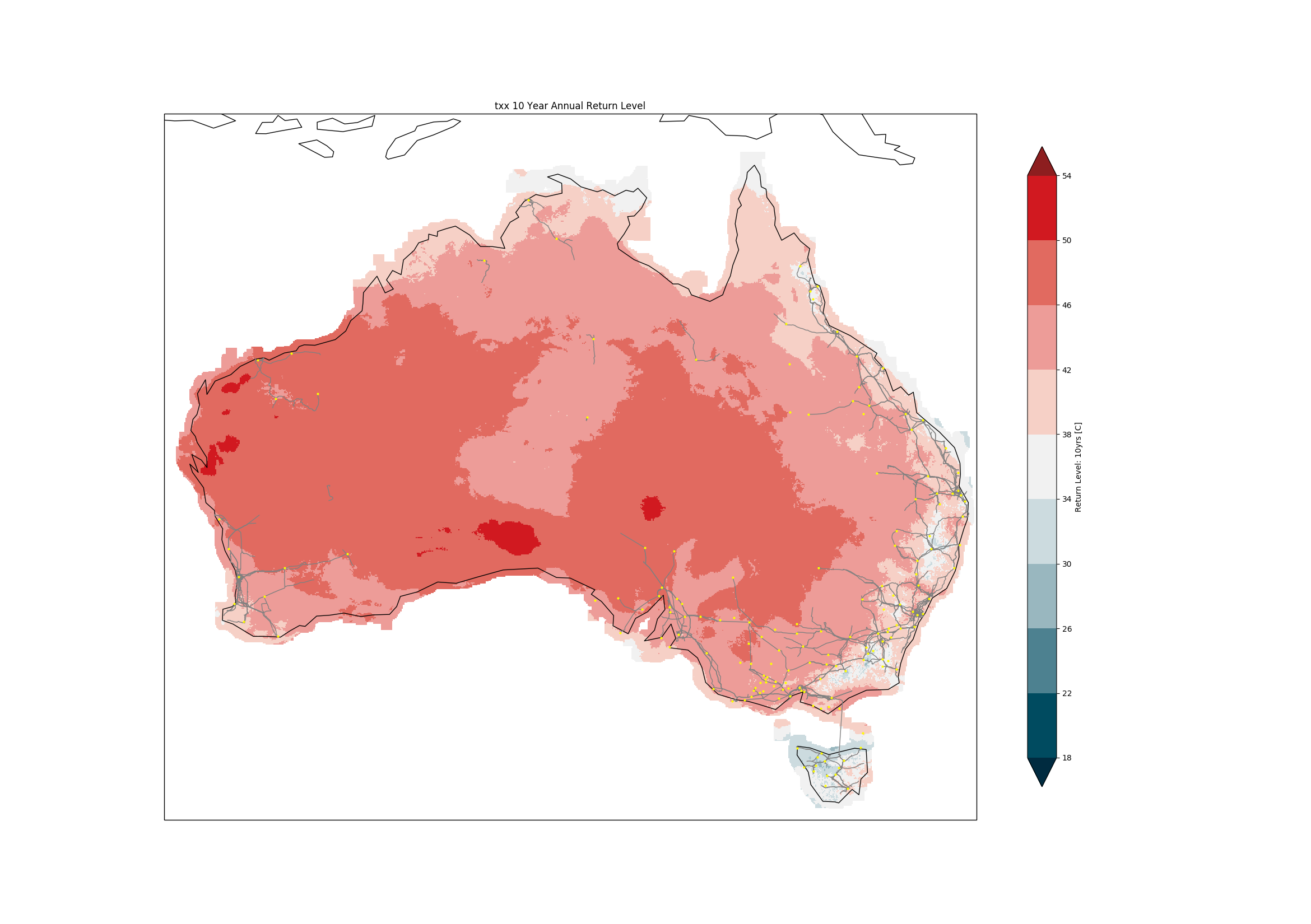
When analysing extremes for multiple variables, to ensure internally consistency between projected changes, data should be derived from individual climate model simulations. Single model ARI-10 is shown in Figure 1 for daily maximum temperatures from three model simulations. Other variables could be derived from the same models to provide internally consistent data for risk assessments.
Sample maps of ARI-10 outputs
| 2020-2039 | 2060-2079 | ||
|---|---|---|---|
(a) GFDL-ESM2M-CCAM (warm dry) |
 |
 |
|
(b) CanESM2-NARCliM-j (hot) |
 |
 |
|
(c) ACCESS1.0-BARPA (mid case) |
 |
 |
|
(d) NorESM1-M-CCAM (warm wet) |
 |
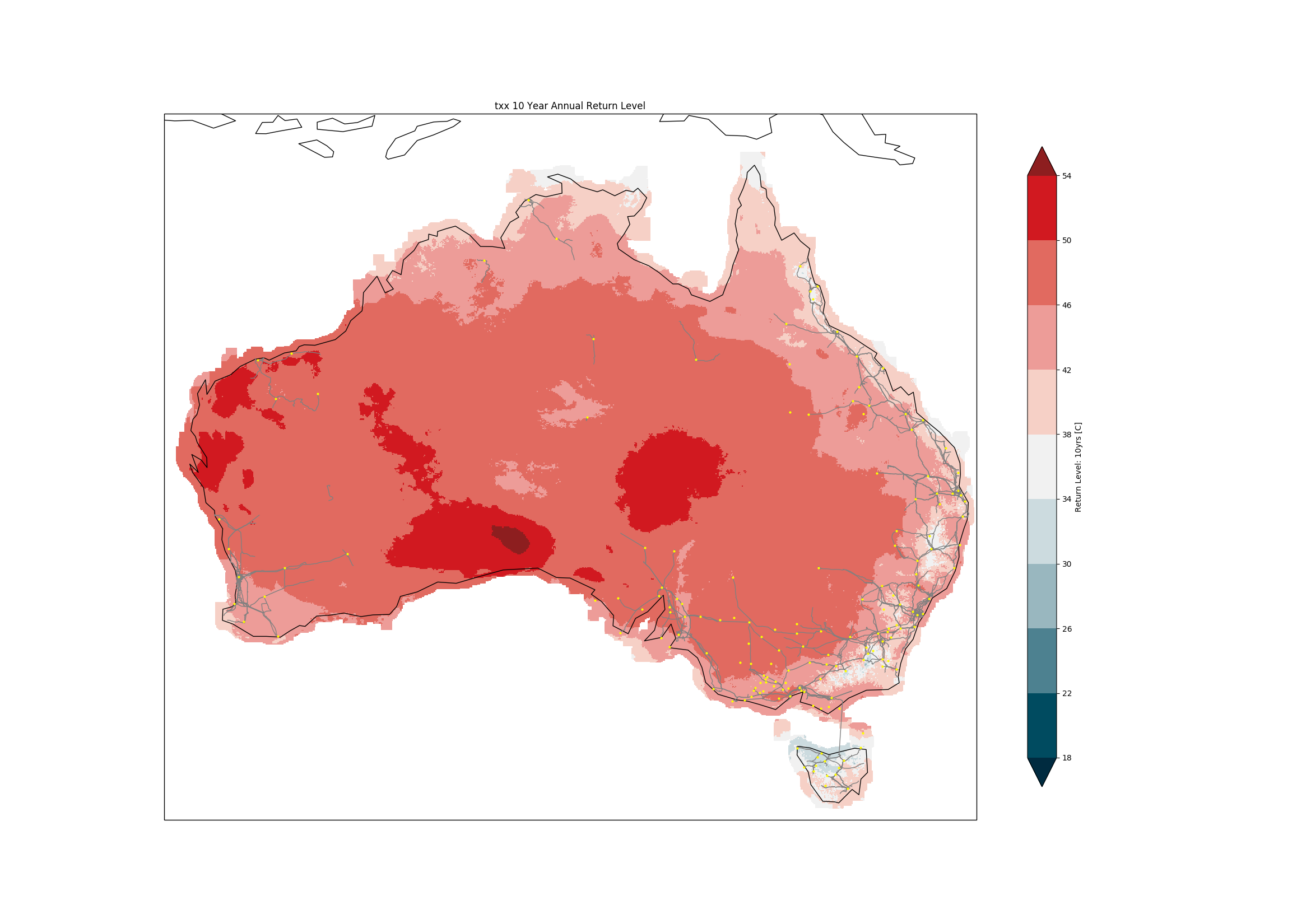 |
Figure 1 ARI-10 of daily maximum temperatures derived from the four ESCI recommended data sets (a) 'warm dry' model GFDL-ESM2M downscaled using the CCAM RCM, (b) 'hot' model CanESM2 downscaled using the NARCliM-j RCM, (c) 'mid-case' model ACCESS1.0 downscaled using the BARPA RCM (note, this RCM is not currently available for WA) and (d) 'warm wet' model NorESM1-M downscaled using the CCAM RCM. All models have been bias-corrected using QME. Two periods are plotted for comparison: the 20 year period centred on 2030 and the 20-year period centred on 2070.
Notes
1 Note: the methodology means that gridded ARI projections are not actually 'maps' in the usual sense that one cell can be compared with the next because the value at any point is derived from an ensemble of downscaled climate simulations and the values at adjacent grid point may come from different models.
2 For more information on the climate models used by the ESCI project and recommended data sets see ESCI Key Concepts—ESCI recommended data sets—testing and validation.
Downloads
DownloadSample ARI-10 Maps (zip 2.1 MB)
ESCI Recommended Data Sets – Testing and Validation
- Summary
- Available Datasets
- 1. Detailed Weather and Climate Data Including Information About Extremes
- 2. A Recommended Subset of Data
- Important Notes
- Key Aspects of the Recommended Data Sets
- References
- Downloads
Summary
Regional climate changes are simulated by climate models in response to increases in greenhouse gases. Models are our best tools for integrating the complex processes and producing physically plausible projections. Dozens of climate models are available, each with strengths and weaknesses. There isn't a single 'best' model, but the ESCI project has identified a subset of models that perform well over Australia and represent most of the range of projected changes in key climate variables such as temperature, rainfall, wind and fire danger.
The ESCI project recommends that detailed impacts analysis should use as a starting point: two global greenhouse gas concentration pathways (moderate and very high) and output from at least four selected climate models. Data from the selected models are post-processed using a technique that is specialised for calibration including of extreme weather events, and three of the models have additional regional insights produced by high-resolution regional downscaling. These recommended data sets provide a minimum standard that can be used in most risk assessments, enabling consistency and comparability. They are relevant to the electricity sector and are scientifically credible.
Data for other climate models, including high-resolution regional downscaling, are also provided and can be used to supplement the recommended data sets; it is always good to use as many of the model outputs as possible to explore more of the plausible ‘uncertainty space’ in climate change.
Available data sets
All climate data available through the ESCI project are based on the Coupled Model Intercomparison Project phase 5 (CMIP5) global climate models (GCMs) used globally, including in the Intergovernmental Panel on Climate Change (IPCC) Fifth Assessment Report.1 The ESCI project recommends using two greenhouse gas concentration pathways, RCP4.5 (moderate) and RCP8.5 (very high).2,3 Collaboration between electricity sector stakeholders and climate scientists identified two key needs; detailed data sets about extreme weather events in future climates, and a recommended minimum set of projections to use in risk assessments.
1. Detailed weather and climate data including information about extremes
Many risk analyses for the electricity sector need climate change scenarios that are detailed in space and time, including insights on extreme events. This is especially needed for assessing electricity reliability risk (e.g. stress testing). This need is addressed by the provision of 16 detailed climate projections for two greenhouse gas concentration pathways. The projections feature:
- The use of high-resolution regional climate models (also known as ‘dynamical downscaling’) to complement the use of global climate models—producing detailed outputs with the potential for valuable new regional-scale information on climate.4
- The outputs from global climate models and from regional climate models were both augmented by a post-processing technique tailored specifically for extremes called Quantile Matching for Extremes (Dowdy 2020) which produces data sets that are ‘application ready’ (free of bias compared to observed data sets, including for extremes) and appropriate for the analysis of changes to averages as well as extremes at the daily time scale.
The 16 climate projections use a common set of seven GCMs as input, selected as they perform well in the Australian region (noting ACCESS-1.3 was found to have some notable biases), and represent a broad range of projected climate change. The projections use three different high-resolution regional modelling systems: CCAM, BARPA and NARCliM.
These 16 projections complement and add to the climate projections for four greenhouse gas concentration pathways and over 40 GCMs (with limited post-processing not tailored for extremes) available on the Climate Change in Australia website. The 16 projections are (Table 1):
- Four simulations from GCMs, with QME post-processing.
- One simulation from the Bureau of Meteorology Atmospheric high-resolution Regional Projections for Australia (BARPA) model with QME post-processing.
- Six simulations from the NSW and ACT Regional Climate Modelling project v1.5 (NARCliMv1.5), with two model configurations labelled J and K, with QME post-processing.
- Five simulations from the CSIRO’s Conformal Cubic Atmospheric Model (CCAM), with QME post-processing.
| Method | ACCESS 1.0 | ACCESS 1.3 | CanESM2 | CRNR-CM5 | GFDL-ESM2M | MIROC5 | NorESM1- M | Spatial scale | Temporal scale* |
|---|---|---|---|---|---|---|---|---|---|
| GCM-QME | ✔ | ✔ | ✔ | ✔ | 5 km | Daily | |||
| BARPA-QME** | ✔ | 5 km | 30 min | ||||||
| NARCliM-QME | J and K | J and K | J and K | 5 km | 60 min | ||||
| CCAM-QME | ✔ | ✔ | ✔ | ✔ | ✔ | 5 km | 30 min |
* Note that QME post-processing produces daily data. Sub-daily data are also available, but they exclude QME post-processing.
** Note BARPA is not available for Western Australia and for RCP4.5 at present.
2. A recommended subset of data
It can be time-consuming and complex to deal with data from many different models, so there is a need for a recommended minimum data set. This is addressed by considering the strengths and weaknesses of the data sets, and the range of projected climate change in each, then recommending a subset of four models that sample key uncertainties and can be used in most risk assessments. This allows consistent and comparable analysis across the sector.
The four recommended models are a subset of the 16 projections produced by ESCI: two CCAM, one NARCliMj, and one BARPA. All are post-processed using QME, and available for RCP4.5 and RCP8.5 (except ACCESS1.0-BARPA-QME, which is only available for RCP8.5—if RCP4.5 is needed, ACCESS1.0-QME can be substituted).5 The four models are a broadly representative of the projected changes from the wider set of 16, and the larger set of over 40 CMIP5 models, in terms of average temperature (Figure 1) and rainfall (Figure 2).
Dynamical downscaling can change the regional pattern of projected change compared to the host GCM, by simulating processes at a finer scale and allowing for regional effects such as rainfall over mountain ranges. In the four recommended models, the downscaling largely follows the host GCM’s projected changes, with some notable exceptions over mountain ranges or areas such as Tasmania, which are likely to be a result of ‘added value’).6 One other important difference is that the south-east of Australia is drier in CCAM compared to the NorESM1-M model used as input (see Figure 2, right column). This is also likely to be due to ‘added value’ and is a better resolution of the effects of changes in atmospheric circulation and weather systems.
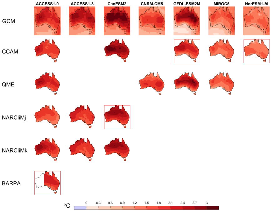
Figure 1 Difference in annual average temperature between 1986–2005 and 2040–2059 under the very high concentration pathway RCP8.5 based on a set of seven CMIP5 models (columns) for the different downscaling techniques (rows). The four recommended cases are outlined in red, noting especially CanESM2 downscaled using NARCliMj is typically hot, and NorESM1-M downscaled using CCAM is typically at the cooler end, with the other two in between. Note: BARPA doesn’t cover Western Australia.
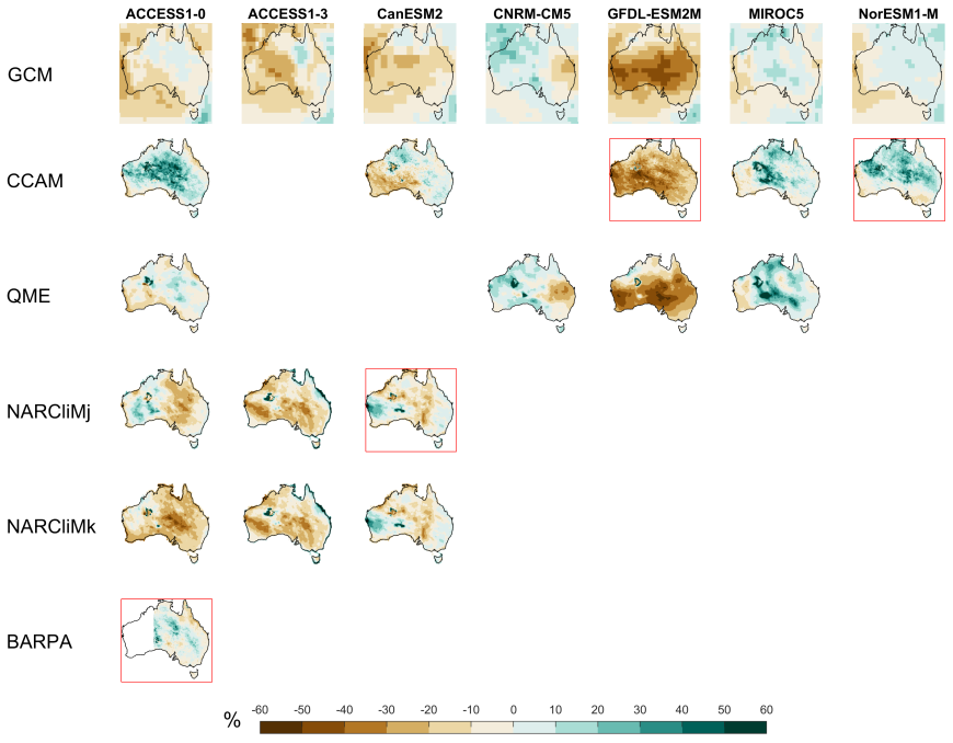
Figure 2 As for Figure 1, but showing annual average rainfall change, noting especially GFDL-ESM2M downscaled using CCAM is a dry projection, and NorESM1-M downscaled using CCAM is at the wetter end except for southern Australia, the other two generally sit between these two.
The four projections can be considered representative of four futures, described by general terms like hot, wet, dry, warm (Table 2). The ACCESS1.0 model simulation downscaled through BARPA gives a middle of the range projection for most regions and variables. The GFDL-ESM2M model downscaled using CCAM is at the warm–dry end of the model range, with rainfall changes of –20 to –30% for much of Australia for 2050 under RCP8.5. The NARCliM-j simulation using CanESM2 is at the hot end of the range of models in all regions, with little change in rainfall, and the NorESM1-M model downscaled using CCAM is at the warm–wet end of projections in most cases. The changes can also be viewed in relation to the wider range of 40 GCMs in scatterplots of temperature and rainfall change (Figure 3). Note that the four models span much of the CMIP5 range in each case but not the entire range—a subset of just four models can’t achieve this. Other cases can be used to supplement these four: for example, in southern Australia, CanESM2-CCAM-QME (a hot future), and MIROC5-QME (warm future with little change in average rainfall) can be used.
| No. | Global climate model | Downscaling model | Northern Australia | Southern Australia | Eastern Australia | Inland (Rangelands) |
|---|---|---|---|---|---|---|
| 1 | GFDL-ESM2M | CCAM | Warm, Dry | Warm, Dry | Warm, Dry | Warm, Dry |
| 2 | CanESM2 | NARCliM-j | Hot | Warm | Hot | Hot |
| 3 | ACCESS-1.0 | BARPA | Mid case | Mid case | Mid case | Mid case |
| 4 | NorESM1-M | CCAM | Warm, wet | Mid case | Warm, wet | Warm, wet |
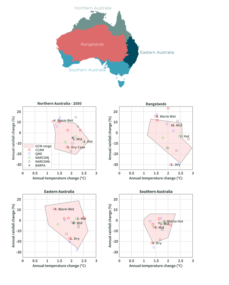
Figure 3 Projected change in annual temperature and rainfall between 1986–2005 and 2040–2059 under very high emissions pathway (RCP8.5) for four broad regions of Australia shown in the map. The polygon shows the range simulated by 40 GCMs in CMIP5 as reported in Climate Change in Australia, the markers show the 16 ESCI projections, differentiated by symbol. The four suggested models are noted by the number and general description from Table 2.
Different models give different changes to average wind speeds (Figure 4), including larger changes from NARCliM than other models. Fire weather measured by the Forest Fire Danger Index (FFDI) generally increases everywhere, with some exceptions, as shown in Figure 5 for the change in the annual average FFDI (July–June). FFDI changes generally follow the changes in the input variables temperature, rainfall and wind (see a direct comparison in Figure 6 for CCAM).
The analysis described here shows changes to the climate averages, or the ‘mean state’ of the climate. Changes to other heat-related variables, such as extremely hot days, follow changes in mean temperature. Change in moisture-related variables, including some extremes such as drought and soil moisture, as well as cloud and solar radiation, generally follow changes in mean rainfall. So, the changes in mean temperature and rainfall are useful dimensions to classify projections for many purposes. Some climate changes, such as changes to storms or damaging winds, may not follow these two variables.
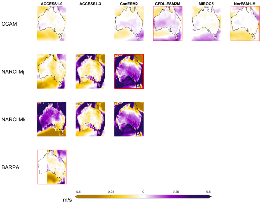
Figure 4 As for Figures 1 and 2 but showing surface wind speed, only dynamically downscaled projections shown (note changes are larger for the NARCliM simulations).
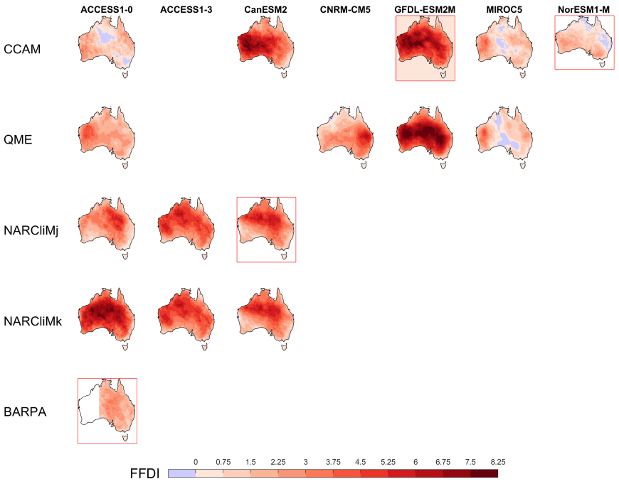
Figure 5 As for Figures 1 and 2, but for change in average annual FFDI.
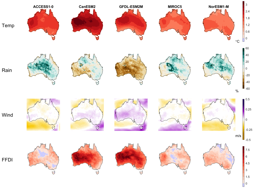
Figure 6 Projected change in annual mean temperature (°C), rainfall (%) wind speed (m/s) and forest fire danger index (FFDI) between 1986–2005 and 2040–2059 under the very high concentration pathway (RCP8.5) from the five GCM-CCAM-QME projections, showing how changes in all input variables contribute to changes in FFDI (e.g. NorESM1-M shows lower temperature change, increasing rainfall and little change in wind speed on the east coast—providing a ‘little change’ FFDI scenario, whereas CanESM2 in central Western Australia shows higher temperature change, decreasing rainfall and an increase in wind speed, so an increase in FFDI).
The ESCI Technical Report on downscaling and testing data sets for a complete report on the evaluation of the ESCI data sets (ESCI, 2021).
Important notes
See ESCI Glossary for definition of terms
1. These climate projection data sets represent plausible future scenarios, but they are not deterministic or probabilistic predictions; it is always good to use as many model outputs as possible to explore more of the plausible ‘uncertainty space’ in climate change.
2. Different choices of greenhouse gas pathways, global climate models and post-processing model outputs, and whether to downscale the projections dynamically, will produce different results—there is no one ‘authoritative’ version of plausible future climate scenarios. More model outputs than this minimum set should be considered whenever possible, to test the effect of choices on the outcome.
3. The data sets are post-processed to be consistent with historical data at the daily timescale—this means they will be relatively free of bias at the daily, monthly and annual timescales. Data sets with a sub-daily timestep are also available from dynamical downscaling (e.g. hourly), but these are not post-processed and should be used only with expert support.
Key Aspects of the Recommended Data Sets
Consider two greenhouse gas pathways suggested by ESCI—data sets use two greenhouse gas concentration pathways—moderate (RCP4.5), consistent with global warming of less than 2 °C since pre-industrial until at least mid-century, and very high (RCP8.5), consistent with 3–5 °C global warming (or more) by 2100.7 The two selected RCPs are useful for a range of resilience and reliability applications. Note the very low pathway (RCP2.6) would result in similar projections to RCP4.5 up to the year 2050, but weaker projections and lower impacts than RCP4.5 after 2050. RCP2.6 is very relevant for analysing ‘transition risks’.8
Evaluated—the recommended data sets draw on global climate models that pass evaluation tests for Australia. The recommended dynamical downscaling also passes evaluation tests (ESCI 2021).
Fully described, internally consistent—data sets are taken from individual simulations from climate models (rather than combining outputs from multiple models, or other techniques). This means the outputs are a coherent representation of the climate system at the scale of daily variability, inter-annual variability and multi-decadal climate change. It also means climate variables such as temperature, rainfall, wind speed and fire danger are internally consistent and can be used for multi-variable risk analysis (e.g. all else being equal, wetter is cooler with lower fire danger and drier is hotter with higher fire danger for a given day, year or climate change case).
Detailed in space and in time—dynamical downscaling produces fine temporal detail (e.g. hourly data) and spatial detail (12–50 km) and gives the potential to ’add value’ to the climate change projection (e.g. enhanced warming and/or drying near notable features of topography). The QME post-processing produces outputs with a fine spatial scale (5-km grid) and a daily timestep that accounts for regional effects represented in the observations (historical data from the Bureau of Meteorology). Note the spatial and temporal detail added by post-processing and regional modelling doesn’t mean that the broadscale climate change (e.g. the change in processes such as El Niño Southern Oscillation) are more accurate or plausible than the global model used.
Consistent for changes to averages and extremes—employing a post-processing technique with a special focus on extremes (QME) ensures that daily statistics are unbiased and realistic for daily extreme values. Dynamical downscaling also produces averages and daily extremes in a consistent way. Important note: as mentioned above, sub-daily data sets are provided in raw form (not post-processed).9
Representative of the projected range of change—recommended data sets are selected to show a range of possibilities that are representative of the broader scientific assessment of climate change (described in Climate Change in Australia, and the IPCC Fifth Assessment Report), and the range of change produced by the broader range of models. Please note that any subset of four recommended models is a balanced compromise between fully representing projected changes (in multiple seasons, regions or variables) and minimising the complexity of data sets that can be used in risk assessments. There will always be plausible changes in some seasons, regions or variables that are not fully captured by the subset.
References
Dowdy AJ (2020). ‘Seamless climate change projections and seasonal predictions for bushfires in Australia’ Journal of Southern Hemisphere Earth Systems Science 70(1):120–38 https://doi.org/10.1071/ES20001
ESCI (2020). Technical Report on downscaling and testing data sets.
Notes
1 See Key Concept—New data sets available from CMIP6.
2 See Key Concept—Choosing representative emissions pathways (RCPs).
3 See Key Concept—Scaling data for RCP2.6 (and other uses).
4 See Key Concept—Climate models and downscaling.
5 Note: ACCESS1.0-BARPA-QME for RCP 4.5 will be available through the Australian Climate Service and may be added to the ESCI project website in due course.
6 See Key Concept—Climate models and downscaling.
7 See Key Concept—Choosing representative emissions pathways (RCPs).
8 See Key Concept—Scaling data for RCP2.6 (and other uses).
9 Sub-daily data from CCAM was used in the following ESCI Case Studies: Extreme heat & VRE, Bushfire & transmission.
Downloads
DownloadAll figures (zip 4.3 MB)
National Hydrological Projections
- National Hydrological Projections
- The Hydrological Projections Approach
- Hydrological Projections Products
- Available Climate Information on Streamflow from the ESCI Project
- References
- Contact
- Downloads
National Hydrological Projections
The Australian Water Outlook is a seamless water resource assessment service by the Bureau which will be released shortly. The service provides nationally consistent information on key water balance components ranging from historical (since 1911 to present), to forecast (short-term and seasonal) and projections time scales (out to 2099). The service is underpinned by the Australian Water Resource Assessment (AWRA) model, the Bureau's operational, national hydrological model—running daily on a ~5-km grid (Frost, Ramchurn, and Smith 2018). The AWRA-L model is calibrated to and evaluated for a wide range of climate conditions resulting in a set of common parameters that represent hydrology over a large range of climate, geological and vegetation conditions to provide soil moisture, runoff and evapotranspiration outputs.
The Hydrological Projections Approach
The Hydrological Projections project provides information on changes of key water balance components—rainfall, runoff, potential evapotranspiration, and soil moisture for multiple future periods in comparison to a historical reference period (1976–2005). The climate data used to run the future AWRA-L model simulations stem from four General Circulation Models (GCMs) and one Regional Circulation Model (RCM), CCAM. The GCM and RCM outputs were bias- corrected using three statistical methods (Figure 1). Additionally, the AWRA-L model was run with bias corrected BARPA (the Bureau of Meteorology’s RCM) outputs for east Australia.

Figure 1 The Hydrological Projections data processing workflow.
The climate variables output from the GCMs, including rainfall, temperature, wind speed and solar radiation, are produced from CMIP5 (Coupled Model Intercomparison Project Phase 5 CMIP5 ), and the regional climate model CCAM model (Rafter et al. 2019). The climate models chosen were a subset of the climate change projections for Australia (projections ), which have been reviewed rigorously to reflect Australian climate conditions as accurately as possible. The selection criteria for inclusion into the NHP data set required that the GCMs must be able to (1) model key physical interactions and processes that are known to be important for Australia's climate; (2) capture the full range of future change across CMIP models (i.e. both wetter and drier responses); and (3) include all variables required to run the hydrological simulations using AWRA-L available at daily scale. The climate outputs from the GCMs and RCMs were re-gridded to a ~5-km grid using a remapping algorithm. As target data set for the bias-correction, climate observations from the Australian high-quality spatial climate Australian Water Availability Project data set (AWAP; Jones, Wang, and Fawcett 2009) were used. Three bias-correction methods were applied, two uni-variate methods and one multi-variate method: (1) the univariate Quantile Matching for Extremes method (QME, Dowdy 2020, also used for the ESCI recommended datasets) adjusts for climate extremes; (2) the Intersectoral Impact Model Inter-comparison method (ISIMIP2b) preserves long-term trends and adjusts for dry days (Hempel et al. 2013); and (3) the Multivariate Recursive Nested Bias Correction (MRNBC) method incorporates the interaction among variables across daily, monthly, and annual timescales to improve representation of low frequency variability (Johnson and Sharma 2012).
An intensive evaluation process investigated the mean bias trend as well as spatial and temporal variabilities of mean and extreme conditions to understand the influence of the bias correction and downscaling step on climate variables and hydrological outputs.
Hydrological Projections Products
Hydrological change information based on the hydrologic projections dataset will be made available via a user interface (UI). The UI will present the median absolute and relative hydrological changes over 30-year time aggregates centred around 2030, 2050, 2070 and 2085, for annually and seasonally aggregated data. The graph panel on the UI will show the spread of the 16 ensemble members. Aggregated data on hydrological change will be downloadable as charts or tables. The application-ready, bias-corrected climate data sets as well as the daily-scale hydrological projections from each of the 16 ensembles and two emission scenarios are available via the NCI Data Collection. A set of hydrological change assessment reports including key messages providing insights into the complex nature of hydrological change complements the Hydrological Projections service. The applicability of the projections data set is showcased by a demonstration case including guidance material and an uncertainty analysis for the use of long-term water asset planning.
Available Climate Information on Streamflow from the ESCI Project
The ESCI project has worked with the National Hydrological Projections project to produce climate information tailored to the needs of the electricity sector. This includes • Projections of the change factors for streamflow for Hydrological Reference Station catchments in 20-year increments for both individual climate models and for an ensemble of climate models (ensemble median, 10th and 90th percentile). This information can be used as a quick assessment of whether changing hydrological conditions is likely to present a risk.
- ARI maps of soil moisture changes for time periods to 2100, and time series at 168 locations around the national electricity market for a suite of climate models.
- Time series for changes in streamflow for Hydrological Resource Stations (HRS) and for catchments around the NEM are available upon request. These projections are available for several individual climate models and can be used to construct an ensemble which captures uncertainty in future climate projections.
- Rainfall projections are provided using ESCI downscaled datasets providing changes as both gridded data (maps) and as time series at 168 locations around the NEM.
This information is available through the ESCI portal on Climate Change in Australia. Gridded, daily hydrological projections data is available via NCI Data Collections and the data can be made available upon request.
References
Dowdy AJ (2020). ‘Seamless climate change projections and seasonal predictions for bushfires in Australia’ (2020) Journal of Southern Hemisphere Earth Systems Science 70:120–38. https://doi.org/10.1071/ES20001
Frost AJ, Ramchurn A, and Smith A (2018). The Australian Landscape Water Balance model (AWRA- L v6). Technical Description of the Australian Water Resources Assessment Landscape model version 6.
Hempel S, Frieler K, Warszawski L, et al. (2013). ‘A trend-preserving bias correction—the ISI-MIP approach’ Earth System Dynamics 4(2):219–36. https://doi.org/10.5194/esd-4-219-2013
Johnson F and Sharma A (2012). ‘A nesting model for bias correction of variability at multiple time scales in general circulation model precipitation simulations’ Water Resources Research 48(1). https://doi.org/10.1029/2011WR010464
Jones DA, Wang W, and Fawcett R (2009). ‘High-quality spatial climate data-sets for Australia’ Australian Meteorological and Oceanographic Journal 58:233–48.
Rafter T, Trenham C, Thatcher M, et al. (2019): CCAM Climate Downscaling Data for Victoria 2019. v2. CSIRO. Service Collection. http://hdl.handle.net/102.100.100/77939?index=1
Contact
Dr Ulrike Bende-Michl, Bureau of Meteorology
email: Ulrike.Bende-Michl@bom.gov.au
Downloads
Download
Figure (png 958.1 KB)
New Data Sets Available from CMIP6
- New Data Sets Available from CMIP6
- New Emissions Pathways
- Performance of Models
- Projected Change
- References
- Downloads
New Data Sets Available from CMIP6
A new group of global climate model simulations from around the world is being evaluated and will become the new international standard following milestones such as the Intergovernmental Panel in Climate Change (IPCC) Sixth Assessment Report in 2021–2022. This means a shift of usage in the science community from the Coupled Model Inter-comparison Project phase 5 (CMIP5) to the new phase, CMIP6. There are many more models available from CMIP6 compared with CMIP5 and many more simulations (or ‘ensemble members’).
The ESCI project used CMIP5 models because the new CMIP6 model ensemble is not ‘mature’ enough for use in a project with the sophistication of ESCI. Specifically:
1. After they are run, new climate models need to be carefully assessed and compared—this process is ongoing. It was not possible to make considered decisions about the prudent use of CMIP6 during the ESCI project.
2. ESCI requires detailed data sets, so downscaling of CMIP5 global climate models, that had been thoroughly evaluated over the Australian region, was carried out using regional climate models to add value. It was not possible to downscale CMIP6 models during the ESCI project.
Since the new CMIP6 models will attract more and more attention through 2021 and 2022, and there will be interest in how the results compare to what is presented in ESCI, some basic context and details are given here.
New Emissions Pathways
The CMIP5 projections were produced for the Representative Concentration Pathways (RCPs): RCP2.6, RCP4.5, RCP6.0 and RCP8.5; the number representing the increase in climate forcing (solar energy retained by the earth in Watts per square metre) by the year 2100.1 The projections in CMIP6 are done under an updated set of future pathways—the Shared Socio-economic Pathways (SSPs; O’Neill et al. 2014). There are five SSPs representing different future worlds (Table 1), and each one is compatible with a range of climate forcing, given as the second number, for example 2.6, 4.5, 7.0, 8.5. Even though the second number in the SSP is the same as an RCP, the SSPs are updated pathways with a different starting point, evolution through time and mix of gases. There are many possible combinations of SSP and forcing, however four ‘Tier 1’ combinations are the highest priority and will have detailed model datasets to support them.
| SSP | Range of Forcing (W.m-2) | Tier 1 SSP |
|---|---|---|
| SSP1 – Sustainability | 1.9 to 6.0 | SSP1–2.6 |
| SSP2 – Middle of the Road | 1.9 to 7.0 | SSP2–4.5 |
| SSP3 – Regional Rivalry | 2.6 to 7.0 | SSP3–7.0 |
| SSP4 – Inequality | 2.6 to 7.0 | – |
| SSP5 – Fossil-fueled Development | 2.6 to 8.5 | SSP5–8.5 |
Performance of Models
The CMIP6 models show incremental improvements in the simulation of the climate of Australia and the broader region (Grose, Narsey, Delage, et al. 2020). However, the fundamental nature of the models hasn’t changed and many of the same biases largely remain. This means that confidence in the projections is mostly similar but may be incrementally higher in some cases—or greater detail in projections may be more confidently reported.
Projected Change
The projected changes in CMIP6 are generally similar to CMIP5. The new set of models do not contradict or invalidate the findings from CMIP5 but rather produce some new detail and new insights on top of the previous models.
The CMIP6 ensemble contains a large group of models with high temperature projections for a given emissions pathway, as these models have a higher value of ‘climate sensitivity’ (how much the global temperature increases when carbon dioxide is increased). This needs some further attention to deal with this appropriately. When standardising and sampling models for a given global warming level, the results between CMIP5 and CMIP6 are very similar.
Projected changes to many other key variables are also similar between CMIP5 and CMIP6, but with some new insights available from CMIP6. For example, projected annual rainfall change under a very high emissions pathway (RCP8.5 or SSP5–85) show many of the same aspects—high model agreement for decrease in annual rainfall in southern Australia, particularly south-west Western Australia, but less certain direction of change for places such as northern Australia (Figure 1).
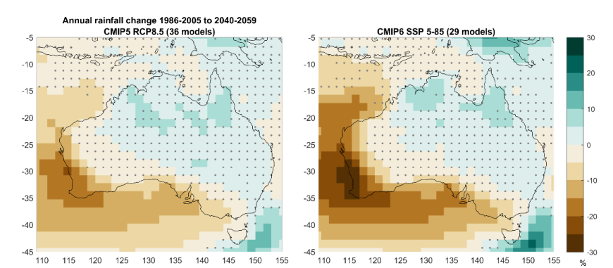
Figure 1. Projected change to average annual rainfall between 1950–1999 and 2050–2099 under a very high emissions pathway (36 models for RCP8.5 in CMIP5; 29 models for SSP5–85 in CMIP6), showing the multi-model mean rainfall change, with stippling (dots) indicating where less than two-thirds of the models agree on the direction of change—there is high agreement on increase at the equator, but lower agreement elsewhere in both model groups—but perhaps more agreement in CMIP6 in some key regions.
References
Grose MR, Narsey S, Delage FP, et al. ‘Insights from CMIP6 for Australia's Future Climate’ (Apr 2020) Earth's Future 8: e2019EF001469
O'Neill BC, Tebaldi C, van Vuuren DP, et al. ‘The Scenario Model Intercomparison Project (ScenarioMIP) for CMIP6’ (2016) 9(9) Geoscientific Model Development 3461–82. https://gmd.copernicus.org/articles/9/3461/2016/
Notes
1 See ESCI Key Concept—Choosing representative emissions pathways.
Downloads
Download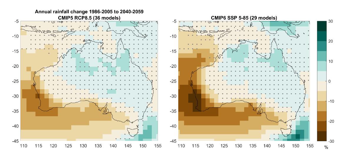
Figure (png 112.7 KB)
Scaling Data for RCP2.6
- Introduction
- Method 2: Scaling Using Change Factors
- Method 3: Rule of Thumb in Time Periods (RCP2.6 Only)
- Confidence in the Future Data Sets
- Downloads
Introduction
The ESCI project has developed a range of data sets for use in risk assessment which use greenhouse gas emissions pathways for two future climate scenarios, RCP4.5 and RCP8.5.1 However, there may be times when additional data are required for a different emissions pathway. Due to limited availability of key data, the ESCI project did not produce future data for the lowest emissions scenario, RCP2.6, but if this pathway is required for the risk analysis there are a number of ways to obtain usable data sets.
Method 1: If only high-level information is required (e.g. figures, tables, statements), then projections material available on the CCiA website www.climatechangeinaustralia.gov.au , produced using CMIP5 models can be used, including Technical Reports and web tools. These data and information products are readily accessed so are not described further here.
Method 2: If you need general-use data sets for a variety of cases, then a process of simple scaling using change factors from the website can be used—see detailed instructions below.
Method 3: If you need detailed data which is consistent with the detailed ESCI data sets used for RCP4.5 and RCP8.5, that is consistent model choice, downscaling method and QME post-processing, then a simple ‘rule of thumb’ to map from higher RCPs to the lower one in terms of time periods can be used—see below.
Method 2: Scaling Using Change Factors
2.1 Variables
Decide what variables are required. The method used to produce the future scaled data is determined by whether the risk assessment requires consideration of just one climate variable in isolation, or more than one variable, used together.
Consideration of a single variable is often appropriate when doing a ‘first pass’ or ‘scan’ type of assessment. For example, if assessing the risk of network substations reaching critical temperature thresholds in future, it may be appropriate to consider maximum temperature only.
When it is necessary to use multiple variables in combination, it is critical that the combination of the projected change for each variable is physically plausible (or ‘internally consistent’). In such cases, data for each variable should be obtained from the same model. (This process can be repeated to obtain a spread of risk analyses for a number of models.)
Both approaches are described further below.
2.2 Temporal Resolution (‘season’)
Decide what season or temporal resolution is important for the risk assessment. For example, if the system of interest only fails in summer, it is likely to be appropriate to use just summer data. In other cases, data for individual months or annual averages may be appropriate.
2.3 Obtain Observed Data
In most cases, appropriate data can be obtained from the Bureau of Meteorology (BoM) Climate Data Online website. Sometimes you may have access to other observed data sets, such as from data loggers.
It is critical to ensure the observed data used for scaling represents the historic period relevant to the projected changes. For projections based on the CMIP5 global climate modelling (including most ESCI data), the observations should be from 20 or 30 years, centred on 1995. For many locations, BoM provides 1981–2010 as a standard period (Figure 1).
Figure 1. Example of climate statistics from BoM Climate Data Online (the link to download the data is circled in red).
2.4 Obtain Projected Change Data
A key source of projection data sets for Australia is the Climate Change in Australia (CCiA) website www.climatechangeinaustralia.gov.au (which also houses the ESCI website).
The choice of data type to use for the projected change information depends on the number of variables to be considered in the risk assessment. Table 1 describes which type of change data to use. The two types are described in more detail in the following sections.
| Number of variables | Change data type | Data source |
|---|---|---|
| One (e.g. maximum temperature not combined with any other variable) | Multi-model ensemble approach: Use values for 10th, 50th (median) and 90th percentiles | CCiA Summary Data Explorer Tool |
| Multiple (e.g. maximum temperature in combination with evapotranspiration) | Individual model approach: In most cases, align with the ESCI recommended representative models (see text). | CCiA Climate Futures Detailed Projections Tool |
2.5 Multi-model Ensemble Approach
Use the Summary Data Explorer tool to obtain projected changes for the region (NRM Sub-Cluster)2 that encompasses the location of interest. Use the ‘CSV’ link to download the data (which can be opened directly in Excel or imported to a range of other software).
Annual and seasonal average change data are available for eight variables (maximum, minimum and mean temperature; rainfall; relative humidity; solar radiation; wind speed; and evapotranspiration) and four future time periods (2030s, 2050s, 2070s and 2090s) under RCP2.6, RCP4.5, RCP6.0 and RCP8.5.
2.6 Individual Model Approach
Use the Climate Futures Detailed Projections tool to obtain the change data from the individual models of choice. In most cases, it will be appropriate to use the GCMs aligned with the ESCI recommended models (Table 2). Alternatively, the Detailed Projections tool can be used to identify appropriate representative models.
| ESCI Recommended Model | CCiA GCM |
|---|---|
| GFDL-ESM2M- CCAM-QME (Warm Dry) | GFDL-ESM2M |
| CanESM2-NARCliM-j-QME (Hot) | CanESM2 |
| ACCESS1.0-BARPA-QME Mid case (Mid case) | ACCESS1.0 |
| NorESM1-M-CCAM-QME (Warm Wet) | NorESM1-M |
Change data are available for four RCPs (RCP2.6, RCP4.5, RCP6.0 and RCP8.5) and for 13 future time periods (2025, 2030, 2035, . . ., 2090). Note that not all the ESCI recommended models are available for RCP2.6 and RCP6.0. For the worked example below we will use RCP2.6, but the same process can be used for other RCPs.
More information on the Climate Futures tool is available on the CCiA website along with the online User Guide .
2.7 Apply Projected Changes to Observations for RCP2.6
Use the change values you have obtained to modify your observed data to produce plausible future values consistent with RCP2.6. The method used to combine the observed and future data depends on whether the change data are provided as ‘absolute change’ (e.g. +1.5 °C) or ‘relative change’ (e.g. +10%). Table 3 describes the formula used to scale using each of these change types.
| Example observed data | Change data to use | Scaling formula |
|---|---|---|
| Average maximum temperature for Jan (°C) | DJF (Summer) or Jan (°C change) | Future Jan temperature in °C = Observed temperature in °C + Change in °C |
| Average minimum temperature for Jul (°C) | JJA (winter) or Jul (°C change) | Future Jul temperature in °C = Observed temperature in °C + Change in °C |
| May–Oct average rainfall (mm) | MJJASO (May–Oct; % change) | Future MJJASO rain in mm = Observed rain in mm x (change in % / 100 + 1) |
| April average rainfall (mm) | MAM (autumn) or April (% change) | Future April rain in mm = Observed rain in mm x (change in % / 100 + 1) |
| Daily maximum temperature3 from 1/1/1981 to 31/12/2010 | Jan change (°C) for Jan days, Feb change for Feb days, etc. | Future daily max temperature in °C = Observed temperature in °C + corresponding monthly change in °C |
This should be repeated for each time frame of interest to give you a time-series for your variable(s) consistent with RCP2.6 (or other pathway).
Method 3: Rule of Thumb in Time Periods (RCP2.6 Only)
RCP2.6 represents a case where global warming plateaus during the 21st century, at around 2050. The change to regional climate also plateaus in many respects—including the change to regional temperature and rainfall averages and extremes and change to many other types of climate extremes remain fairly constant in 2050–2100. However, some aspects of the climate do not plateau when warming plateaus, such as regional sea level rise, which will continue for some time even if temperature stabilises. For most applications except sea level, the following rule of thumb can be used:
RCP2.6 in 2050 onwards (due to the plateau) is roughly equivalent to:
- the climate under RCP4.5 in 2030–2050, or 2040–2060 if 2030–2050 is unavailable
- the climate under RCP8.5 in 2020–2040
Further future periods for RCP4.5 and RCP8.5 move more and more outside this window, as follows:
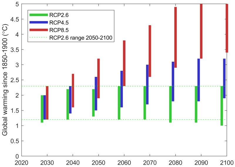
Figure 2 Global warming projections in 20-year periods for the CMIP5 global climate models.
Following global warming, the regional changes in many other variables also show this same approximate equivalence in time periods. However, the effect can be obscured by regional scale variability. For example, there is high confidence in a significant decline in south-west Western Australian spring rainfall, but the dry end of projected change is more limited under RCP2.6 than under the higher RCPs. Using RCP4.5 in 2050, or RCP8.5 only in 2030, as proxies for RCP2.6 throughout the century is appropriate as it avoids the changes of > 30% only projected under higher RCPs later in the century.
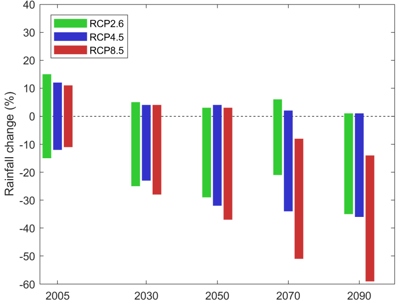
Figure 3 South-west Western Australia spring rainfall change in 20-year periods for the CMIP5 global climate models.
Confidence in the Future Data Sets
The ESCI Technical Report on the Standardised Methodology for Projections Likelihood describes the ‘multiple lines of evidence’ approach used for assigning confidence statements to CCiA projections.4 It is important to understand that different climate variables will have different confidence statements associated with them. For example, rainfall projections are generally of lower confidence than temperature projections.5 When scaling is used to produce future climate data, the confidence statement associated with the relevant projected change data should be carried through to the future data.
Notes
1 Representative concentration pathways (RCPs) have been developed by the international climate change research communities to describe how the future may evolve. More information can be found in ESCI Key Concepts —Choosing representative emissions pathways (RCPs).
2 Natural Resource Management (NRM) clusters are regions of the country where the climate is expected to change in the same way at about the same rate.
3 This approach is appropriate for daily temperature data but is not recommended for daily rainfall data.
4 See also ESCI Key Concepts —Climate projection confidence and uncertainty.
5 This confidence information can also be found using the Regional Climate Change Explorer tool and in the CCiA Cluster Reports .
Downloads
DownloadAll figures (zip 357.6 KB)
Using CCiA to Choose Alternative Climate Information
Summary
The CSIRO and the Australian Bureau of Meteorology produced the ‘Climate Change in Australia’ (CCiA) website with funding from the Commonwealth Government’s Regional Natural Resource Management (NRM) Planning for Climate Change Fund, concluding in 2015. The website provides a comprehensive assessment of observed climate change and its causes, climate projections over the 21st century, and guidance on how to use projections in risk assessments.
There is also an extensive library of climate information and data products that can be used to compliment the ESCI climate information and data products. CCiA climate projections are focussed around Natural Resource Management (NRM) regions (Figure 1), and point locations around the country.
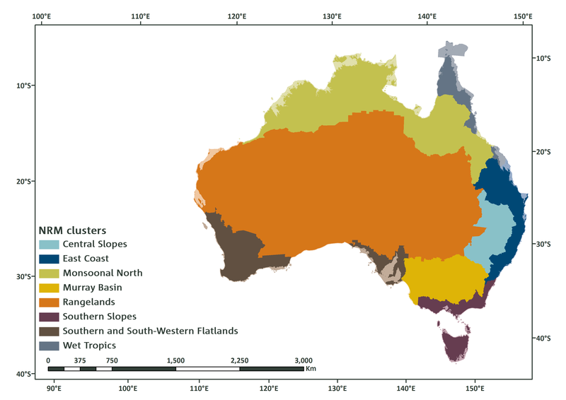
Figure 1. Map of eight NRM cluster regions.
Some useful data sets and tools are available on the CCiA website where you can explore global climate model projections (see below). There is also plenty of supporting information to ensure that you have all the information you need to use the tools and understand the climate model results and visualisations.
Data sets on the CCiA website are available from up to 40 global climate models (including the ESCI recommended models), across three emissions pathways (High; RCP8.5, Mid; RCP4.5, Low; RCP2.6*) (*fewer models represented).
Examples of Tools on the CCiA Website
1. Summary Data Explorer
This interface allows you to explore (and download) the projected changes in eight climate variables for the NRM clusters. In the example below, projected seasonal change in seasonal maximum surface air temperature for the East Coast NRM region (light blue) for four future periods under different emission scenarios RCP2.6 (green), RCP4.5 (blue) and RCP8.5 (purple). Natural climate variability is represented by the grey bar.
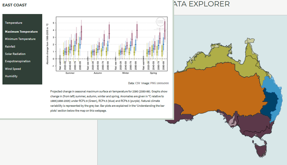
Figure 2 Sample output from the Summary data explorer showing projected temperature changes over the East Coast cluster for four time periods, four seasons and three RCPs (green RCP2.6, blue RCP4.5, mauve RCP8.5).
2. Map Explorer
This tool allows you to produce a map based on selecting a time period, emission scenario, climate variable, climate model and month/season. The default map is the whole of Australia, but sub-regions can also be selected. The output can be displayed as a change relative to the baseline period 1986–2005 or with the changes added to the baseline (Figure 3).
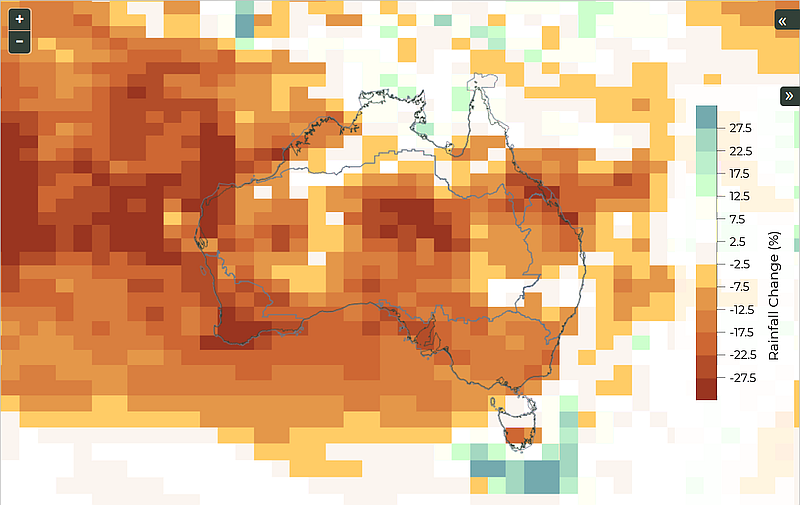
Figure 3. Sample output from the Map explorer for annual mean rainfall change, under RCP8.5 by 2050 for the HadGEM2-CC climate model.
3. Gridded Data Download Tool
Gridded data files can be downloaded using the selected drop-down items shown on the right. Note the options available that may better suit your requirement for projected change information. This example in Figure 4 shows projected maximum temperature change. Future data (changes added to the baseline) are available in gridded format as well (see Data delivery brochure below).
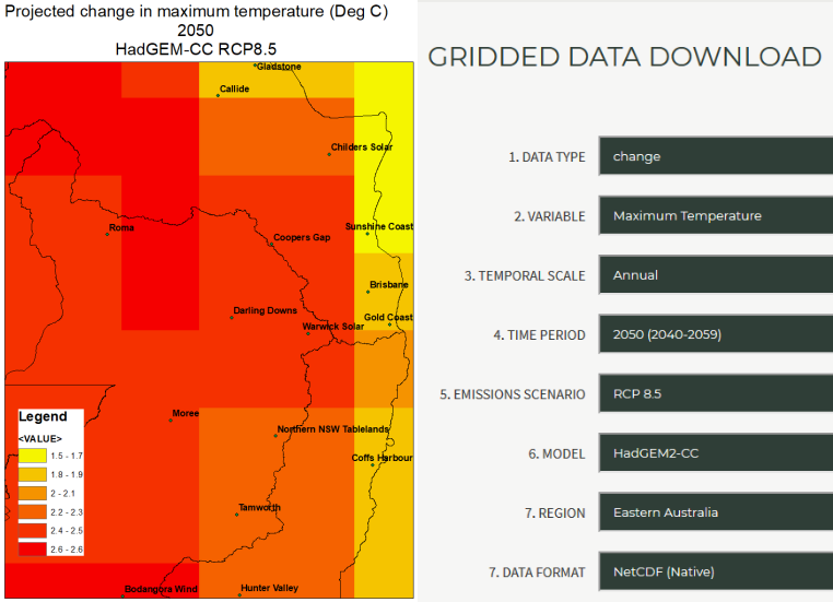
Figure 4 Sample output from the gridded data download function.
4. Thresholds Calculator Tool
The example in Figure 5 shows the average number of days per year with a maximum temperature above 35 °C over Australia for the 2050 (2036–2065) time period (HadGEM2-CC climate model and high emission scenario, (RCP8.5). Mildura threshold exceedance frequencies for 2036–2065 are also highlighted, and can be compared with the historical (1981–2010) exceedance frequency.
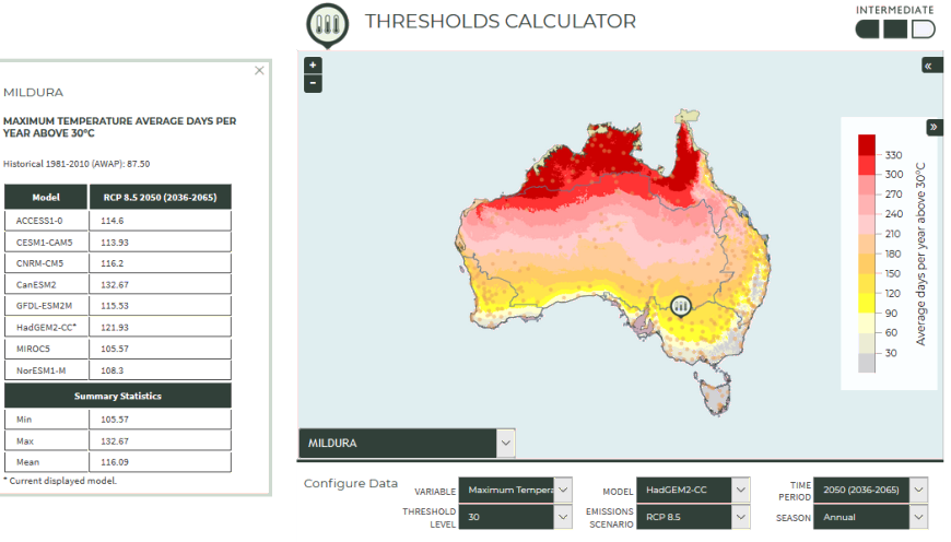
Figure 5 Sample output from the Thresholds Calculator.
More examples of these temperature threshold files can be found here, noting other climate variables and selected thresholds of interest, models and RCPs, and data for individual locations can be viewed and downloaded if required.
5. Time-series Explorer
Time-series data sets enable the user to understand variability and possible trends in a daily, monthly or annual climate sequence. For example, the annual temperature change timeseries is shown for the Murray Basin NRM region in Figure 6. These are available for different climate variables, regions, seasons, across a range of future climate scenarios (eight models/ RCP4.5 and RCP8.5).
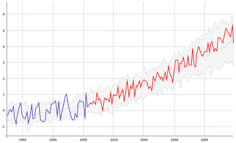
Figure 6 Sample output from the Time-series explorer.
- Grey band (or plume): the range of model results is summarised using the median (central grey line) and 10th to 90th percentile range of the projected change in all 40 CMIP5 simulations.
- Blue line: the historic simulation from the selected model.
- Red line: the future simulation from the selected model.
6. Location Data Download Tool
Projected annual (or seasonal, monthly or daily) time series are available. To create these projected time-series, monthly changes relative to 1986–2005 from the selected climate model and emissions pathway (RCP) are applied to corresponding Bureau of Meteorology high-quality station time-series for 1981–2010. These data are available for Mean temperature, Maximum temperature, Relative humidity (9am, 3pm), rainfall and Pan evaporation (eight models/three RCPs).
Data Delivery Brochure
The CCiA Data Delivery brochure (available in the Downloads section, below) describes the data sources, and their strengths and limitations, and outlines all of the data products available for download from CCiA.
Downloads
DownloadCCiA Data Delivery Brochure (pdf 6.1 MB)