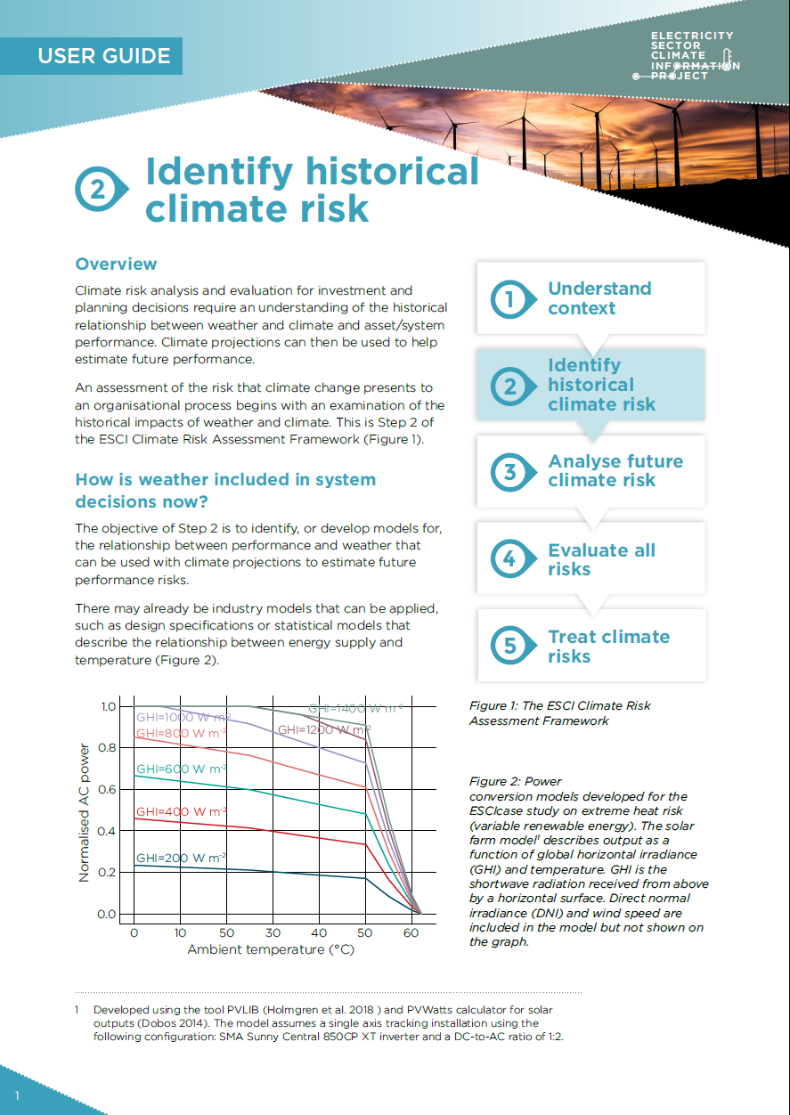
Step 2: Identify Historical Climate Risk

• Overview
• How is weather included in the system decisions now?
• Has an historical relationship between weather and performance been identified?
• Identify important parameters for the risk analysis
• References
• Downloads

Overview

Climate risk analysis and evaluation for investment and planning decisions require an understanding of the historical relationship between weather and climate and asset/system performance. Climate projections can then be used to help estimate future performance. 

An assessment of the risk that climate change presents to an organisational process begins with an examination of the historical impacts of weather and climate. This is Step 2 of the ESCI Climate Risk Assessment Framework (Figure 1).

HOW IS WEATHER INCLUDED IN THE SYSTEM DECISIONS NOW?

The objective of Step 2 is to identify, or develop models for, the relationship between performance and weather that can be used with climate projections to estimate future performance risks.

There may already be industry models that can be applied, such as design specifications or statistical models that describe the relationship between energy supply and temperature (Figure 2).

Figure 1 The ESCI Climate Risk Assessment Framework.

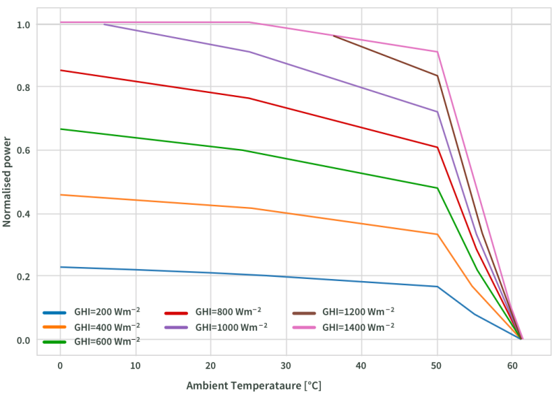
Figure 2. Power conversion models developed for the ESCI case study on extreme heat risk (variable renewable energy). The solar farm model1 describes output as a function of global horizontal irradiance (GHI) and temperature. GHI is the shortwave radiation received from above by a horizontal surface. Direct normal irradiance (DNI) and wind speed are included in the model but not shown on the graph.

HAS AN HISTORICAL RELATIONSHIP BETWEEN WEATHER AND PERFORMANCE BEEN IDENTIFIED?

If industry models do not already exist, building a model that captures the relationship between weather and performance is usually quite straightforward. The impact of weather is already built into many processes and asset specifications. Examples include line ratings based on ambient temperature, and vegetation clearing scheduled during an historically low-bushfire-risk season.

There are likely to be organisational records that relate system impacts to weather. For example, structural failures (Figure 3) can be related to severe convective winds (Figure 4).

The Bureau of Meteorology supplies quality-assured historical weather and climate data.² For each climate variable of interest, try to establish a statistical relationship with historical asset/system performance. This could be a simple linear regression with the fit providing an estimate of uncertainty. Another common statistical method is Monte Carlo analysis which deals with uncertainty through assigning a probability curve of likely outcomes. This can be used wherever there is a range of input data, such as the frequency and timing of a weather event. For example, a transformer’s performance relative to temperature can be calculated using Monte Carlo simulations informed by probability curves based on historical climate information.

Figure 3 Transmission tower structure functional failure history. (Source: AusNet, AMS 10-77 Transmission Line Structures. 2023-27 Transmission Revenue Reset, Section 3)

IDENTIFY IMPORTANT PARAMETERS FOR THE RISK ANALYSIS

Figure 4 Mean historical frequency of conditions favourable for severe convective winds compared with outage events (11 events, 1959–2020). Source: BoM analysis (Brown, 2021) and AusNet Services data used as part of the ESCI Case Study on the risk severe convective winds present to transmission lines.

When identifying historical weather and climate hazards, be specific about hazard thresholds associated with impacts, such as temperatures over 45 ^oC or wind-gusts above 30 m/s. Consider also whether averages or extreme values are most relevant. Identify the temporal resolution that is needed for the historical analysis, as the same resolution (if possible) will be used for future climate analysis. Half-hourly temperature data may be needed for demand modelling and sub-hourly wind data for wind-stress or power modelling. Daily/monthly fire weather data may be most useful, and seasonal streamflow data may be appropriate for hydro-generation modelling.

Spatial scale is also important. Historical weather and climate information may be available only at specific locations, such as Bureau of Meteorology real-time monitoring sites, which provide daily maximum and minimum temperatures. These locations may not be close to your areas of interest, limiting the value of the data. Future climate information is available on a 5-km grid, and as time-series for 168 locations across the national electricity market—check how well these correspond to the locations for historical asset/system performance data sets.³

Once you have developed a model of the relationship between historical climate and asset/system performance, and identified important parameters for the analysis of future risk, then you are ready to move on to Step 3: Analyse Future Climate Risk.

REFERENCES

Brown A and Dowdy A (2021). ‘Severe convection-related winds in Australia and their associated environments’ Journal of Southern Hemisphere Earth Systems Science71(1):30–52. https://doi.org/10.1071/ES19052

Dobos AP (2014). PVWatts version 5 manual (No. NREL/TP-6A20-62641). National Renewable Energy Lab (NREL), Golden, CO. https://doi.org/10.2172/1158421

Hersbach H, Bell B, Berrisford P, et al. (2020). ‘The ERA5 global reanalysis’ Quarterly Journal of the Royal Meteorological Society 146(730):1999–2049. https://doi.org/10.1002/qj.3803

Holmgren WF, Hansen CW and Mikofski MA (2018). ‘pvlib python: A python package for modeling solar energy systems’ Journal of Open Source Software 3(29):884. https://doi.org/10.21105/joss.00884

Notes

¹ Developed using the tool PVLIB (Holmgren et al. 2018 ) and PVWatts calculator for solar outputs (Dobos 2014 ). The model assumes a single axis tracking installation using the following configuration: SMA Sunny Central 850CP XT inverter and a DC-to-AC ratio of 1:2.

² The ESCI project has used the years 1986–2005 as a baseline for climate projections (consistent with the IPCC), but data are available back to 1980 (earlier for hydrology) on the ESCI website.

³ The ESCI project also provides historical and projected summary data for regions with similar climates across Australia.

Downloads