Climate Change in Australia
Climate information, projections, tools and data
Scaling Methods
Detailed explanation of the mean and quantile-quantile scaling methods used
This page summarises the ‘delta change’ or ‘change factor’ scaling methods used to create application-ready data. Either a mean scaling or quantile-quantile scaling method has been used, depending on the generation of GCMs (CMIP6 or CMIP5) and the climate variable (see the tables on the Application-ready data page).
Mean scaling
The essentials of the approach used for mean scaling to create most of the CMIP5 application-ready data are illustrated in Figure 1, below.

Fig.1. An example of the ‘delta change' (or ‘perturbation') method using mean scaling. Here, future climate temperature information (right) is created by adding projected temperature change information from a climate model (middle) to observed data (left).
The steps for producing a mean scaled monthly time-series.
For each 5 x 5 km grid point:
- Calculate historical GCM climatology (20-30 yrs) for each month.
- Calculate future GCM climatology (20-30 yrs) for each month.
- Calculate absolute change by subtracting future from historical for each month.
- Calculate percent change by dividing abs change by the historical for each month.
- For temperature related variables add the absolute change, for all others multiply by the percent change for each month, to data in each month of the observational time-series.
Production of future daily time-series uses the same approach but at the final step, the monthly change value applied is that for the month corresponding to the historic date. For example, in the example shown in Figure 2, a July daily value from the observed data is scaled by the projected change for July.
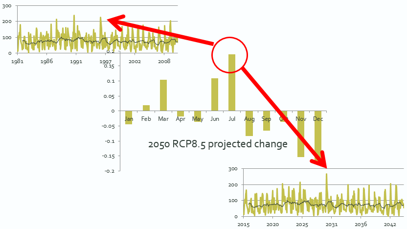
Fig.2. An example showing a daily time-series (top left) being scaled by the appropriate monthly mean change (middle) to produce a plausible future daily time-series (bottom right). The arrows show a July day from the observations being scaled by the July change value to produce the corresponding future daily amount.
Quantile-quantile scaling
Quantile-quantile scaling is a modification to the mean change technique that captures changes in daily variance (see the Technical Report ). Capturing change in daily variance to most important for rainfall. Climate models indicate that extreme daily rainfall intensity and frequency are likely to increase, even in areas where mean rainfall shows little change or a decrease. This represents an increase in daily variance. Capturing this expected change in extreme events in application-ready datasets is very important for future planning. Therefore, quantile-quantile scaling has been used in the production of future daily rainfall data in the CMIP5 application-ready dataset and in the production of data for all variables in the CMIP6 application-ready dataset.
The quantile-quantile scaling methods used differ in detail between the CMIP5 and CMIP6 application-ready datasets.
Quantile-quantile scaling for CMIP5
Step 1: Create quantile-quantile mapping functions for each month from the Global Climate Model (GCM) data (see Figure 3.) The functions are calculated from the 20-year historic baseline period 1986 to 2005 for the future time periods '2030' (2016 to 2045), '2050' (2036 to 2065), '2070' (2056 to 2085) and '2090' (2075 to 2104).
For each 5 x 5 km grid point:
- Rank GCM historical and future daily time-series values from smallest to largest.
- Group ranked values into 10 decile bins, with decile 1 containing the lowest 10% and decile 10 the highest 10% of values.
- To provide more detailed changes in extreme events, divide the 10th decile values into 10 percentile mapping bins, thus giving 19 quantiles (9 deciles plus 10 percentiles) in total.
- Calculate mean values for each decile and upper percentile (quantiles) for both the historical and future data (see Figure 3, bottom left).
- Calculate the change ratio for each quantile by subtracting the historical mean from the future and dividing by the historical (see Figure 3, right).
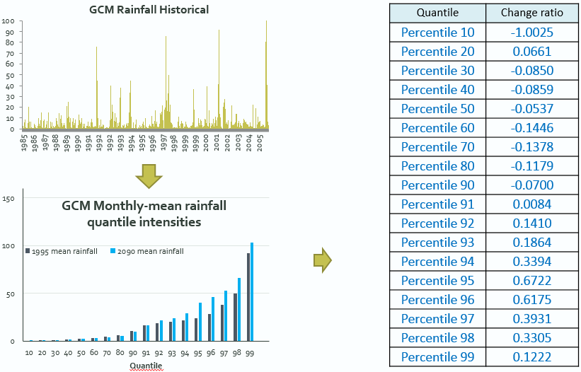
Fig.3. Step 1 of quantile-quantile scaling. GCM simulated historic daily rainfall data (top left) are 'binned' into 19 quantiles (the 100th percentile is not shown). The same is done for the model's future projected times series (bottom left). The change from historic to future is calculated for each 'bin' or quantile (right).
Step 2: Modify Observed data (Figure 4). The observed data used are a 30-year time series (1981 to 2010).
For each 5 x 5 km grid point:
- Rank observed daily time-series values from smallest to largest for each month.
- Group ranked values into 10 decile bins, with decile 1 containing the lowest 10% and decile 10 the highest 10% of values.
- Divide the 10th decile values into 10 percentile mapping bins (20 quantiles total).
- Apply the GCM-based change ratios from each quantile level to all observational values in each quantile. (Multiply the mean change for the GCM quantile by the mean obs quantile value, then add to the obs value).
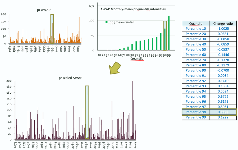
Fig.4. Observed daily rainfall time-series (top left) 'binned' into quantiles (top middle). The quantiles are scaled by the corresponding change ratios (right) and applied to the observations to produce the scaled future time-series (bottom left).
Quantile-quantile scaling for CMIP6
The process for the CMIP6 application-ready dataset (described in detail by Irving & Macadam 2024) is similar to that for CMIP5 application-ready dataset but has some important differences. In addition to using different model data and observations, the most significant methodological differences are:
- Quantile-quantile scaling is used for all variables in the CMIP6 dataset, whereas it is only used for rainfall in the CMIP5 dataset.
- Future time-slice and future global warming level (GWL) data are available in the CMIP6 dataset, whereas only time-slice data are available in the CMIP5 dataset.
- To better sample climate variability, the quantile-quantile mapping functions for the CMIP6 future time-slice data are calculated from a 30-year historic baseline period, 1985 to 2014. For simplicity, the same historic baseline is also used to provide the observed historic baseline for scaling. For the CMIP5 dataset, the 20-year baseline 1986 to 2005 was used to calculate the mapping functions and the 30-year period 1981 to 2010 was used as the observed historic baseline for scaling.
- For simplicity, the CMIP6 future time-slice data includes just two future time periods. These are ‘2050’, or ‘mid-century’, (2035 to 2064) and ‘2085’, or ‘late-century, (2070 to 2099). The CMIP5 dataset included the four future periods '2030' (2016 to 2045), '2050' (2036 to 2065), '2070' (2056 to 2085) and '2090' (2075 to 2104).
- For the CMIP6 dataset, for both the observations and model data, ranked daily values are grouped into 100 percentile bins, whereas 19 bins (9 deciles, plus 10 percentiles covering the most extreme values) are used for the CMIP5 dataset. Percentile 1 contains the lowest 1% and percentile 100 contains the highest 1% of values. This essentially extends the percentile treatment of extreme values used for the CMIP5 dataset to the entire range of values.
- For most variables, the change ratio for each quantile is calculated in the same way for the CMIP6 dataset as for the CMIP5 dataset (i.e., the historical quantile mean is subtracted from the future quantile mean and then dividing by the historical quantile mean). The observed values are then multiplied by the change ratios. However, for temperature variables in the CMIP6 dataset, absolute changes in quantile means are used (i.e., the historical quantile mean is simply subtracted from the future quantile mean). These absolute changes are then added to the observed values.
Important notes regarding the time-series datasets
The future time-series produced are 30-years in duration. They are intended to be representative of the projected climate state for that time. For this reason, it is not appropriate to join the separate time-series together to build a plausible continuous time-series for the whole 21st Century (see Figure 5).
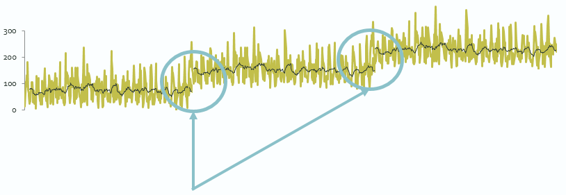
Fig.5. Illustration of the discontinuity in consecutive future time-series datasets. For the CMIP5 application-ready data the actual time-series datasets overlap more than indicated. For the CMIP6 application-ready data the actual time-series datasets do not overlap.
Important notes regarding the GWL datasets
A global warming level (GWL) represents how much the global-mean surface temperature has increased since the pre-industrial (1850-1900) period. The standard practice is to use a 20-year period corresponding to when the 20-year centred average of the global-mean surface temperature first reaches a particular value / level (see global warming levels – methods for details). Following this practice, a baseline of GWL 1.0 °C was used to produce application-ready data corresponding to GWL 1.5 °C, 2.0 °C, 3.0 °C and 4.0 °C using data from combining the CMIP6 historical and SSP3-7.0 experiments. The 20-year period corresponding to the GWL 1.0°C baseline (and indeed any other GWL) differs for each model (Figure 6). For example, the 20-year periods corresponding to GWL 1.0 °C and 2.0 °C were 2003-2022 and 2029-2048 respectively for the ACCESS-CM2 model. Producing application-ready data for GWL 2.0 °C involved calculating the quantile changes between 2003-2022 and 2029-2048 from the ACCESS-CM2 data and then applying those changes to observed data from 2001-2020, which is the GWL 1.0 °C period in observations. It should be noted that a small number of GCMs do not reach 4.0 °C of global warming by the end of the century, so GWL 4.0 °C data was not provided for those models (Figure 6).
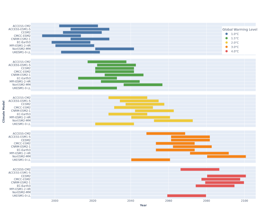
Fig. 6. The 20-year period corresponding to various global warming levels for the models used in the CMIP6 application-ready dataset.
Page updated: 1st Dec 2025
