common mistakes when using climate change data

There are some common mistakes users make when working with climate projections data for an impact assessment. Some mistakes, and suggested ways to avoid these are listed below:

Not representing an appropriate range of climate model output. MORE

Climate projections are produced from up to 40 models, so there is a range of results to consider. It is not always practical to conduct an impact assessment using the result from all available models, therefore it is recommended to carefully select models that represent a range of possibilities.

Not representing, nor discussing, the range of plausible emission scenarios. MORE

The future pathway of greenhouse gas and aerosol emissions during the 21st century is uncertain. The four scenarios used for climate projections represent a range of plausible futures. Choice of scenarios (and hence rate of climate change) in an impact assessment can have a large influence on the potential results. See Important considerations for more information.

Not respecting the integrity of modelling output.

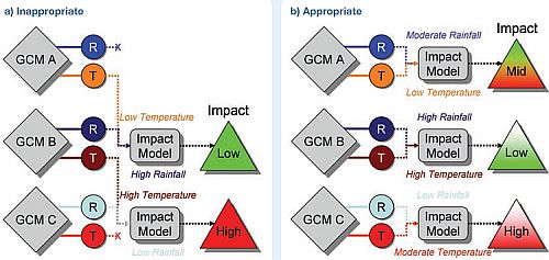
Climate data within an individual climate model has internal consistency, i.e. correlations between climate variables are physically plausible, as are the simulated changes. Mixing data from different climate models does not respect the integrity of data from individual climate models. For example, it is inappropriate to use temperature (T) data from one model and use rainfall data from another model in an impact assessment (see Figure a). This may lead to a physically implausible combination of climate data. However, it is appropriate to use data for multiple variables from an individual model in each impact assessment (see Figure b).

Example of appropriate and inappropriate use of climate model projections in impact assessment.

For both figures (a) and (b), rainfall (R) and temperature (T) projections from three different global climate models (GCMs) are applied in a hypothetical impact model. In (a), each pair of global climate model scenarios is applied independently to the impact assessment model, resulting in a range of different climate impacts that may be misleading. In (b), projections of rainfall and temperature from different models are paired to yield internally consistent scenarios of climate change, which are then applied to the impact model.

Not checking model evaluation results.

Model evaluation provides information on how well climate models represent historical climate and forms an integral part of the confidence rating process for climate change projections. The assumption is that good performance from a particular model over the historical (1986-2005) period increases reliability of the projected changes. Chapter 5 in the Technical Report discusses global climate model evaluation for the Australian region.

It is important to check the model evaluation results to ensure that a model with low performance over a certain region is not used (or used with caution).

Assuming results from downscaled studies are always better and/or more relevant, and not understanding the limitations of downscaling methods.

Dynamical or statistical downscaling of information from global climate models (GCMs) offers more detailed information about climate change.

Dynamical downscaling involves the use of fine resolution atmospheric models (driven by output from global climate models), opening up the possibility for a more accurate depiction of key processes, especially in regions with complex topography. Statistical downscaling involves applying observed statistical relationships (between large-scale and local climate) to large-scale changes in climate simulated by models in order to estimate changes at local scales. 

However, downscaling doesn’t always provide a superior projection of change for a given region. There are numerous issues to contend with: selection of GCMs for downscaling, pros and cons of different downscaling methods, representation of the physical processes that drive change, internal consistency of projected changes across multiple variables, as well as practical issues around handling large datasets. Some regions offer greater potential for downscaling to add value to projections from global climate models, so this is where downscaled projections should be considered for impact assessment.

Not understanding the temporal and spatial limitations of global climate model.

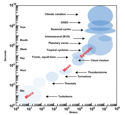
Most climate models in the latest generation of global climate models (CMIP5) have a spatial resolution (horizontal) of around 200 km. Whilst spatial resolution in both the horizontal and vertical direction have become significantly finer over time, at this scale some physical climate processes can still not be resolved. This means that some local or regional climate affects are not always simulated by the models. Model evaluation can help to develop a deeper understanding of which models are better performers. Likewise downscaling of GCMs can be used, where appropriate, to give finer scale projections encompassing regional climate features. There is significant computational expense associated with increasing spatial (and temporal) resolution of global climate models. In some cases and for some processes it is not possible to provide reliable quantitative projections.

Space and time-scales of dynamical atmospheric processes. SOURCE: UCAR

Attributing all recently observed weather and climate extremes to anthropogenic influence.

Formal attribution has typically been based on research that uses a combination of climate modelling, instrumental climate observations, physical understanding and sometimes palaeoclimate reconstructions (use of proxies such as tree rings and ice cores to establish climate over Earth’s history) to investigate cause and effect in a climate change context.

Extreme event attribution is more challenging than attributing long-term changes. Extreme weather occurs naturally, with and without the influence of humans. Furthermore, these are rare (by definition). Most events are not exclusively due to either human or natural causes but some combination of both.

However, methods have been developed to quantify the role of human and other external influences on these specific extreme events.

Further reading on attribution:

CHRISTIDIS, N., STOTT, P., KAROLY, D. & CIAVARELLA, A. 2013. An attribution study of the heavy rainfall over eastern Australia in March 2012 [in “Explaining extreme events of 2012 from a climate perspective”]. Bull. Amer. Meteor. Soc, 94, S58-S60.

KING, A. D., ALEXANDER, L. V. & DONAT, M. G. 2013. The efficacy of using gridded data to examine extreme rainfall characteristics: a case study for Australia. International Journal of Climatology, 33, 2376-2387.

LEWIS, S. C. & KAROLY, D. J. 2013. Anthropogenic contributions to Australia's record summer temperatures of 2013. Geophysical Research Letters, 40, 3705-3709.

Assuming model or image resolution is proportional to accuracy.

Some statistical methods can make maps look more accurate through re-gridding to a finer scale. It is important to note that bi-linear interpolation, the process used to re-grid the maps in the following figure, does not add extra information about climate change and therefore the finer resolution map (right) is not more accurate than the coarser resolution data (left). Pay close attention to the mapping technique used in spatial representations of future climate change.

Example of bi-linear interpolation where finer resolution (right) is not actually more accurate that the coarser resolution data (left).

Confusing projection and prediction.

Descriptions of future regional climate are usually referred to as ‘projections’ (or ‘scenarios’, see below). Projections have a range of uncertainty for a given a climate variable due to differences between the results of various climate models. A climate change ‘projection’ is also conditional on the choice of emission scenario. This conditionality is the primary reason a projection is not called a ‘prediction’. A prediction estimates the sequence of events in the future, including the effects of both climate change AND variability (see figure).

Figure shows the difference between observations, predictions and projections.

Assuming the level of confidence in climate projections does not vary for different variables/ regions/ or time periods.

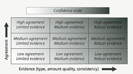
Confidence language has been specified by the Intergovernmental Panel on Climate Change (IPCC) for their Fifth Assessment Report which considers factors along two dimensions; evidence (type, amount, quality and consistency), and agreement between those lines of evidence. A confidence rating can be assigned using calibrated language based on expert judgment of the various lines of evidence (see Figure). As in IPCC, confidence is expressed using the qualifiers ‘very high’, ‘high’, ‘medium’, ‘low’ and ‘very low’.

A depiction of evidence and agreement statements and their relationship to confidence as described by the IPCC. Confidence increases towards the top right corner as suggested by the increasing strength of shading.

Confidence ratings differ between climate variables. For example there is very high to high confidence that temperatures and sea levels will increase, but medium confidence for projections of tropical cyclones.

In setting confidence ratings, the simulated range of change from CMIP5 models (and any consistency on the direction of change simulated) is considered and supplemented by information obtained from the following lines of evidence;

1. Model reliability at simulating relevant aspects of the current climate
2. Results from relevant downscaled projections
3. Evidence for a plausible process driving the simulated changes
4. The level of consistency with emerging trends in the observations.

For rainfall change, model results can vary in direction and magnitude, so all of these lines of evidence should be considered in some detail (as is done in the Technical Report Section 7.2). Some other variables described in this report did not always permit or require this full approach, but in all cases confidence is assessed and reasons are given.