How does a climate model work?

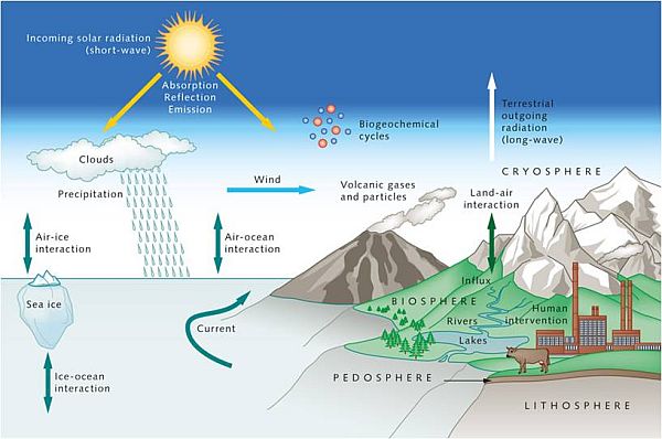
Global climate models are mathematical representations of the Earth’s climate system, based on the laws of physics and run on powerful computers. They represent fundamental physical processes in the atmosphere, ocean, land surface and cryosphere. 

Theoretically, these physical processes can be represented mathematically even though there is some chaotic behaviour involved at small scales (e.g. droplet interactions within clouds). Some of the challenges in developing an Earth system model are that:

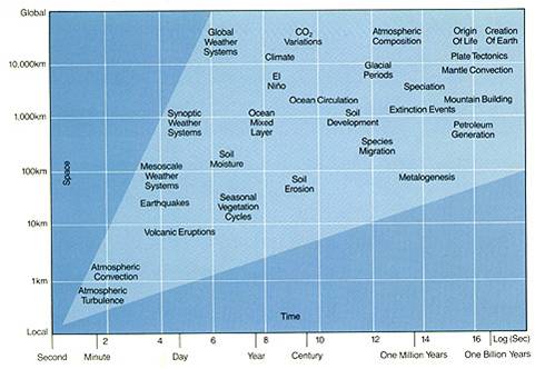
(a) many processes making up the Earth's climate operate on different temporal and spatial scales (see figure below) from a few metres and seconds to thousands of kilometres and thousands of years; and

(b) these processes interact with each other across different time and space scales. This means that even though a global climate model is mainly used for decadal-to-century long projections, they seek to incorporate as many short-term and small scale processes as possible since these also interact with the larger scales.

Schematic of the time scale across which different Earth system processes act

With respect to temporal scales: at each model time step, a new state of the Earth’s atmosphere and oceans is calculated and then used as the initial state for the next time step. By this method the model is ‘stepped forward’ in time. The simulated climate can then be inferred by the ‘statistics’ (averages, extremes etc) from multi-decadal simulations. Typical global climate model time steps are 30 minutes up to 3 hours – meaning that processes that happen on shorter time scales are not captured per se but must be parameterised (or approximated). This is similar for spatial scales: with typical spatial resolution of 200km (for the atmosphere) for each grid cell of the model, processes that are smaller in scale (e.g. condensation of water vapour into cloud droplets), are not simulated per se but are parameterised. Physical aspects are complemented by other empirical equations that describe other elements of the Earth system and how they interact, for example the effect of vegetation cover.

A significant constraint is the cost involved in running such complex models. Usually run on powerful super computers, the costs are not only the runtime, but also the infrastructure necessary for storing such large data amounts.

Despite these limitations, global climate models have complex representation of important physical processes and manage to produce quite realistic daily weather, seasonal variability and long term climate states.

Schematic of Earth system interactions

For climate change experiments, it is important that models capture the fundamental processes that respond to climate ‘forcing’ (e.g. the radiation changes from changing greenhouse gases and aerosols). Consequently some of the important parts of a global climate model relate to:

1. The response to variability of solar irradiance on a range of time scales.
2. Changes to the Earth's energy balance at the surface and top of atmosphere from volcanic eruptions
3. How radiation is absorbed and reflected on its way through the atmosphere but also at the surface.
4. Atmosphere and ocean dynamics (and how energy and momentum is transported through the different media)
5. How greenhouse gases and aerosols affect the Earth's climate and climate variability
6. Sea ice and polar ice sheets
7. Various climate ‘feedback’, such as the interaction of clouds and water vapour with the warming climate, and the changing absorption or emission of CO₂ from the ocean and land surface.

climate models and weather forecasts

While there are many similarities between models used for daily weather forecasts and models used for climate projections, there are some important differences. The IPCC (2013) notes:

To make accurate weather predictions, forecasters need highly detailed information about the current state of the atmosphere. The chaotic nature of the atmosphere means that even the tiniest error in the depiction of ‘initial conditions’ typically leads to inaccurate forecasts beyond a week or so. Climate scientists do not attempt or claim to predict the detailed future evolution of the weather over coming seasons, years or decade.

Some types of naturally occurring ‘internal’ variability can extend the capacity to predict future climate. If such variability includes or causes extensive, long-lived, upper ocean temperature anomalies, this will drive changes in the overlying atmosphere, both locally and remotely. The El Niño-Southern Oscillation phenomenon is probably the most famous example of this kind of internal variability. Variability linked to the El Niño-Southern Oscillation unfolds in a partially predictable fashion. Meteorological services and other agencies have exploited this. They have developed seasonal-to-interannual prediction systems that enable them to routinely predict seasonal climate anomalies with demonstrable predictive skill.

For multi-decadal projections, historical and 21^st century simulations are required. The historical simulations are initialised in the year 1850 then allowed to evolve until 2005 in line with prescribed forcings, both natural (solar irradiance, volcanic eruptions) and anthropogenic (greenhouse gases, aerosols and land use/cover change) (IPCC, 2013, Chapter 9). Unlike weather forecasts, these historical climate simulations are not periodically adjusted with updated information about the state of the climate to improve the forecast – they are initialised in 1850 then loosely constrained by the prescribed forcing. Therefore, the historical simulations are not designed (or expected) to reproduce the observed sequence of weather and climate events during the 20th century, but they are designed to reproduce observed multi-decadal climate statistics, such as averages. The 21st century simulations run from 2006-2100, driven by prescribed anthropogenic forcings. Owing to uncertainties in the model formulation and the initial state, any individual simulation represents only one of the possible pathways the climate system might follow. To allow some evaluation of these uncertainties, it is necessary to carry out a number of simulations either with several models or by using an ensemble of simulations with a single model, both of which increase computational cost.

Depending on the observational data set, the global mean surface temperature (GMST) trend over 1998–2012 is estimated to be around one-third to one-half of the trend over 1951–2012. For example, in HadCRUT4 the trend is 0.04ºC per decade over 1998–2012, compared to 0.11ºC per decade over 1951–2012. 15-year-long hiatus periods are common in both the observed and CMIP5 historical GMST time series. However, an analysis of the full suite of CMIP5 historical simulations (augmented for the period 2006–2012 by RCP4.5 simulations) reveals that 111 out of 114 simulations show a GMST trend over 1998–2012 that is higher than the entire HadCRUT4 trend ensemble (IPCC, 2013, Box 9.2). This difference between simulated and observed trends could be caused by some combination of (a) internal climate variability, (b) missing or incorrect radiative forcing and (c) model response error.